SGD optimizer with momentum
The optimizer is a unit that improves neural network parameters based on gradients. (I am currently not aware of the optimizer method that is not using gradients).
A good optimizer would train the parameter tensors in a shorter number of steps, compared to the worse one (assuming same accuracy and similar computational time).
The very basic optimizer will do:
\[p_{i+1} = p_{i} - lr * grad_{i}\]In here the parameter $p_{i}$ represents the parameter tensor at batch step $i$, and $grad_{i}$ the gradient tensor at the same batch step and $grad_{i}$ has the same size as $p_i$ tensor.
Check my backpropagation article that shows the process of calculating gradients is not so hard. Also PyTorch training model explains there are the forward and backward passes.
Those two articles explain how and when we calculate gradients in additional detail. In short, we calculate the gradients on backward pass for every mini batch.
A mini batch is a package of items. This may be the package of images, or audios, or text, or gene sequence.
Every mini-batch has a size, and some typical sizes would be 32, 64, 128, but it is OK to train with batch sizes of 1 or 2 if larger batch sizes would lead to memory errors. It is also OK to train with a batch size of 8K or 32K if your hardware allows that.
Shaky Gradients
Since we calculate the gradients of every mini-batch although we don’t know what we may expect inside gradient tensors, we may assume gradients vary from mini-batch to mini-batch.
It would be nice to predict the moving trends for our gradients taking into account every mini-batch so far. This may involve analyzing the average moving gradient.
Since there may be millions or even hundreds of millions of parameters in our neural network it would be demanding to track each gradient for each parameter at each step $i$.
For some applications a simple moving average (SMA) is used. That would calculate the gradient mean based on all previous gradients.
\[{1\over n } \sum_{i=1}^n grad_{i}\]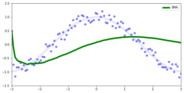
But, this kind of mean doesn’t promptly reflect actual data as we can see in the previous image.
For instance if we have a cos function and some random noise (the blue points) we would expect our prediction to be the transparent blue line, but instead the SMA is a green line.
Luckily there are other techniques.
The exponential weighted moving average EWMA.
EWMA looks like this:
\[a_{i+1} = \beta * a_i + (1-\beta) * grad_{i}\]Here $a_i$ is the average moving gradient. I will show two data models in PyTorch to explain EWMA.
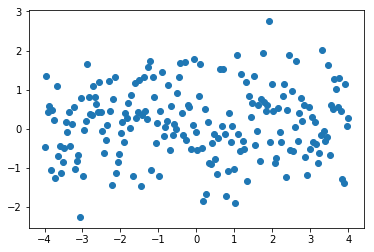
Model 1: Normal data distribution with offset
Let’s consider this normal data distribution for y with offset 0.3.
import torch
x = torch.linspace(-4,4,200)
y=torch.randn(200)+0.3
plt.scatter(x,y)
plt.show()
If we take the next equation to calculate the moving average a:
depending on momentum $\beta$ we may have different results.
In the upper equation we should notice the momentum needs to be carefully set based on what we try to achieve. If we would like to fit almost any data point then the smaller the momentum the better. If we would try to be less bumpy we would consider 0.9 for the momentum.
Model 2: Data distribution is cos function with some noise
Let’s define our data and plot an image:
x = torch.arange(-3.,3.,step=0.05)
x = torch.linspace(-3,3,100)
yo = torch.cos(x) #orig
y = yo + 0.5*torch.rand(yo.size())-0.25
plt.scatter(x,y, alpha=0.5)
plt.plot(x,yo)
plt.show()
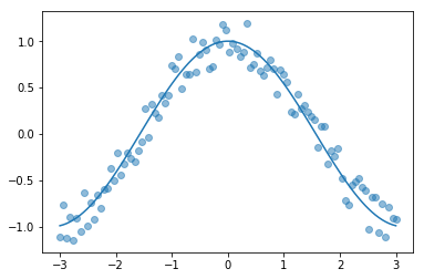
The thin blue line is our cos function. We used it to calculate the scatter plot (the blue dots). Now we are trying to fit on a scatter plot. We use the EWMA again.
Check out that again the momentum $\beta$ plays a huge role on our output. If our momentum is too small like 0.01 we will be far away from the original cosine function.
If you check for the $\beta$ of 0.99 we are still not predicting well, but there is a trick called debiased EWMA.
Debiased EWMA
The trick to create debiased EWMA is to create the EWMA and to divide it by $1-\beta^i$ where, $i$ is our batch number. For the first batch that would be: $1-\beta$, for the second $1-\beta^2$ and so on.
\[a_{i+1} = \frac {\beta * a_{i} + (1-\beta) * grad_{i}}{1-\beta^i}\]where $ a_0 = 0$, $a_i$ is average gradient tensor and $grad_i$ is a gradient tensor.
Creating the new SGD optimizer with momentum
So let’s create a new SGD optimizer with momentum, dampening and debiasing when we know all that.
Original SGD optimizer is just a port from Lua, but it doesn’t have this exact debiased EWMA equation, instead it has this one:
\[a_{i+1} = \beta * a_{i} + (1-dampening) * grad_{i}\]For $dampening = \beta$, this would fit EWMA. Be careful still, because the default $dampening$ is 0 for torch.optim.SGD optimizer.
class SGD(Optimizer):

    def __init__(self, params, lr=0.1, momentum=0, dampening=0  ):
        defaults = dict(lr=lr, momentum=momentum, dampening=dampening  )
        super(SGD, self).__init__(params, defaults)

    def __setstate__(self, state):
        super(SGD, self).__setstate__(state)

    def step(self):

        for group in self.param_groups:
            momentum = group['momentum']
            dampening = group['dampening']

            for p in group['params']:
                if p.grad is None:
                    continue
                grad = p.grad.data
                if momentum != 0:
                    state = self.state[p] # state is dict

                    if len(state) == 0:
                        state['step'] = 0  # batch id
                        avg = state['avg_grad'] = torch.zeros_like(grad)
                    else:
                        state['avg_grad'].mul_(momentum).add_(1 - dampening, grad)
                        avg = state['avg_grad'].div(1-momentum**state['step'])

                    state['step'] += 1

                p.data.add_(-group['lr'], avg)
This code shows several things. It uses the PyTorch Optimizer base class. This means the SGD has parameter state memory for every parameter.
You can check optimizer.state_dict() to check this at any time.
Also, it knows how to deal with param groups. The param group is the idea where we group arbitrary parameters into groups. The only constraint is we cannot feed the same parameter to multiple groups.
Often we create param groups based on the forward execution order.
It is possible to create param groups for all the convolution layers, or for all the linear layers.
The last line of the step method updates the current parameter based on the learning rate and also based on the average gradient.
This last line is the basic gradient descent formula, with our gradient dampened and debiased.
The state['avg_grad'] is what will be preserved for the next step, as this is not what is the avg from the last line of the step method.
This optimizer may be slightly improved for speed considering the ** operation but in general it should behave even better than the original PyTorch SGD.
TODO:
- Consider how it will converge, compared to the PyTorch SGD.
- Consider the impact of batch size.
- Consider accumulating gradients that are close 0 for multiple batches.