PyTorch training model
In here, we have a PyTorch short training model:
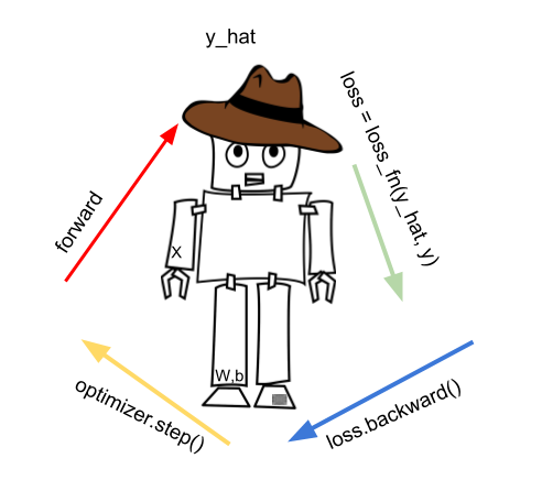
Most notable is the forward pass where we step into the model and predict the y_hat.
We can write this more formally:
y_hat = model(X)
Read: Compute predicted y_hat by passing X to the model.
We define our model, for instance:
model = torch.nn.Sequential(
          torch.nn.Linear(D_in, H),
          # more layers in here ...
          torch.nn.Linear(H, D_out),
        )
The model can be either:
What we get from the model forward phase is the y_hat, or the prediction.
We use that prediction to create the loss, using the loss_fn (the loss function)
loss = loss_fn(y_hat, y)
Sum of all loss values is the error, but we may also say total loss. One of the most common used loss function is the Euclid distance loss:
loss_fn = torch.nn.MSELoss()
Once we calculate the loss we call loss.backward(). The loss.backward() will calculate the gradients automatically. Gradients are needed in the next phase, when we use the optimizer.step() function to improve our model parameters.
We can get all our model parameters via: model.parameters() method. Once we update model parameters, we repeat the forward phase again.
In our example we used the torch.nn.Linear() layer, to transformation the input in linear way (matrix multiplication). A non-linear transformation follows the Linear layer since this is know neural networks can best learn.
Note that each PyTorch forward phase creates the calculation graph; thanks to that graph we compute the gradients…