Variational Auto-Encoder
There are two approaches to inference:
- exact inference
- approximation inference
Variational Auto-Encoders do variational inference thus the name and this is an approximate inference type.
Marginal Likelihood
To perform inference it is sufficient to reason in terms of probabilistic model marginal likelihood which is marginalization of any missing or latent variables in the model. As we will see these will be our $\boldsymbol{z}$ variables.
This integration is typically intractable, and instead, we optimize a lower bound on the marginal likelihood.
VI algorithm is to compute the posterior probability approximately using the neural net.
Probabilistic machine learning
A probabilistic model is a joint distribution of hidden variables $\boldsymbol {z}$ and observed variables $\boldsymbol {x}$:
\[p(\boldsymbol {z}, \boldsymbol {x})\]Inference about the unknowns is through the posterior, the conditional distribution of the hidden variables given the observations:
\[p(\boldsymbol {z} \mid \boldsymbol {x})=\frac{p(\boldsymbol {z}, \boldsymbol {x})}{p(\boldsymbol {x})}\]Question: What is the evidence here?
It’s $p(\boldsymbol x)$, and we should learn this distribution so we can create our own inputs from this distribution.
For the most interesting models the denominator $p(\boldsymbol x)$ is intractable. We can only approximate posterior inference.
Question: What being intractable means?
Bayesian analysis involves computing multidimensional integrals that are often intractable analytically except in a few special cases with conjugate priors.
The other way around is to compute the finite number of integrals, but when there is an infinite number of integrals e.g. in Gaussian mixtures integrals are intractable.
The non Bayesian way with maximum likelihood estimation (MLE) actually is based on computing the derivatives, not the integrals and it is often easier in practice, since we don’t have problems with intractable integrals.
Variational Auto-Encoder assumes:
- input $\boldsymbol x$
- latent space $\boldsymbol z$
- VAE NN parameters $\boldsymbol w$
- PDF of joint $p_{\boldsymbol w}(\boldsymbol x, \boldsymbol z)$ is differentiable
The whole idea of VAE is to create a neural net that approximates the posterior.
Posterior distribution $p(\boldsymbol z \mid \boldsymbol x)$ is the distribution of the latent variable conditioned on the data. This distribution is continuous.
Since we will learn the VAE as neural net, all the neural net parameters are weights so we can rewrite the distribution with respect to the weights: $p_{\boldsymbol w}(\boldsymbol z \mid \boldsymbol x)$.
How VAE works
We start from the input $\boldsymbol x \in \mathbb R^n$, and we encode it not just with $\mathbb E(\boldsymbol{z})$ like in normal autoencoder but we also keep the variance $\mathbb V(\boldsymbol{z})$. Both $\mathbb E(\boldsymbol{z})$ and $\mathbb V(\boldsymbol{z})$ have dimensionality $\mathbb R^d$ so in total after the encoding step we have $\mathbb R^{2d}$.
Encoder : $\mathbb R^n \rightarrow \mathbb R^{2d}$
Decoder : $\mathbb R^d \rightarrow \mathbb R^{n}$
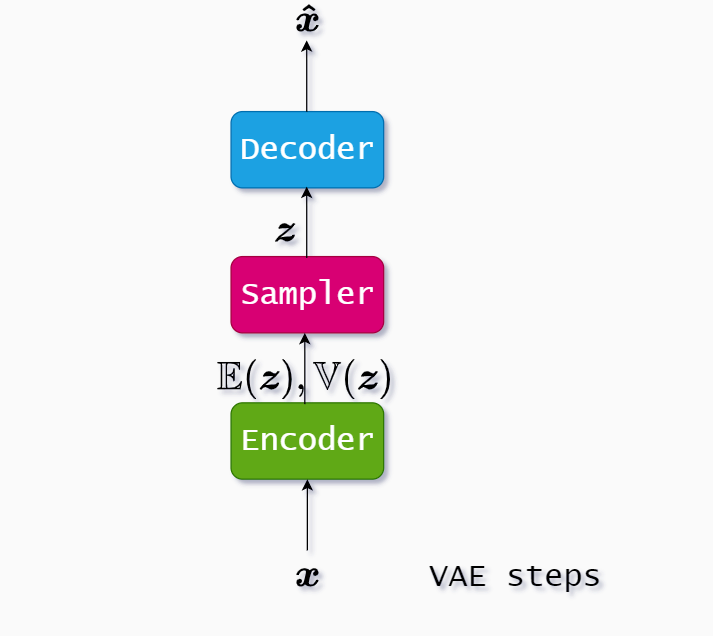
The sampler is capable of creating samples from the Gaussian distribution with $\mathbb E(\boldsymbol{z})$ and $\mathbb V(\boldsymbol{z})$, but we use the reparameterization trick which is to replace the sampler with the equation:
\[\boldsymbol z = \mathbb{E}(\boldsymbol{z}) + \boldsymbol{\epsilon} \cdot \sqrt{\mathbb{V}(\boldsymbol{z})} \tag{1}\](1) is called the reparameterization trick since we use addition and multiplication to get the gradients we need for backpropagation.
After we replaced the sampler with reparameterization trick we got $\boldsymbol z$ and lastly we use the decoder to decode the original input, but this time we call it $\boldsymbol{\hat x}$. It should be as close as possible to $\boldsymbol{x}$.
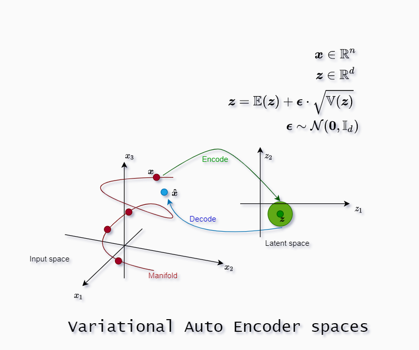
In our image latent space is 2-dimensional $d=2$, and input space is 3-dimensional $n=3$. The green bubble around the point $\boldsymbol z$ denotes the variance.
The manifold is where the inputs live. When we decode values from the latent space we should be as close as possible to the manifold.
Gaussian noise $\boldsymbol \epsilon$
Bayesian would ask now is there some prior distribution used in VAE to regularize the process?
We use simple multivariate Gaussian noise with zero mean vector and identity covariance matrix $\mathbb I_d$, so $\boldsymbol \epsilon \sim \mathcal N(\boldsymbol 0, \mathbb I_d)$. We then write the objective function for VAE:
\[\ell(\boldsymbol{x}, \boldsymbol{ \hat{x}})=\ell_{\text {reconstruction }}+ \ell_{\mathrm{KL}}\left(\boldsymbol{z}, \boldsymbol \epsilon \right) \tag{2}\]or in case we provide hyperparameter $\beta$ to control the relative entropy term:
\[\ell(\boldsymbol{x}, \boldsymbol{ \hat{x}})=\ell_{\text {reconstruction }}+\beta \ell_{\mathrm{KL}}\left(\boldsymbol{z}, \boldsymbol \epsilon \right) \tag{3}\]Since for $\boldsymbol{z}$ we know mean vector and covariance matrix and we know same distribution details for $\boldsymbol \epsilon$, we can calculate analytically the relative entropy formula for those multivariate Gaussian distributions:
\[\beta \ell_{\mathrm{KL}}\left(\boldsymbol{z}, \boldsymbol \epsilon \right) = \frac{\beta}{2} \sum_{i=1}^{d}\left(\mathbb{V}\left(z_{i}\right)-\log \left[\mathbb{V}\left(z_{i}\right)\right]-1+\mathbb{E}\left(z_{i}\right)^{2}\right) \tag{4}\]The sum is due to the fact that the covariance matrix of $\boldsymbol z$ is actually a diagonal matrix (there are no covariances) so we can create a sum of $d$ independent dimensions to calculate relative entropy.
From the references you may find out that since we introduced variance of the latent variable we deal with $d$-dimensional bubbles. Loss function one can see through three meaningful bubble forces:
- $\ell_{\text {reconstruction }}$ force to push bubbles away from each other
- $\mathbb{E}(z_{i})$ force to wrap all bubbles into a single big bubble
- $\mathbb{V}\left(z_{i}\right)-\log \left[\mathbb{V}\left(z_{i}\right)\right]-1$ force prevents bubbles to collapse or explode, keeping bubbles at unit size
References: