NLP progress (brainstorming)
- NLP processing
- BOW
- Co-occurrence matrix
- word2vec
- CBOW
- Skip-gram
- GloVe (Global Vectors)
- The Transformer model
- Tokenizers
- NLP libraries
NLP processing
NLP processing started with regular expressions and with the text normalization methods such as:
- tokenization
- convert words to lower case
- lemmatization
- stemming
Tokenization is splitting sentences into words with optional removal of stopwords, punctuation, words with less than 3 characters, etc.
Lemmatization assumes morphological word analysis to return the base form of a word, while stemming is brute removal of the word endings or affixes in general.
First the statistical NLP methods came along together with the model called Bag Of Words (BOW).
BOW
The BOW idea is to group words together where the order of words is not important and to analyse word frequencies.
Known statistical methods based on BOW are LSA or Latent Statistical Analysis and LDA or Latent Dirichlet Analysis.
With LSA the idea is that if words have similar meaning they will appear in similar text contexts.
It was important because it brought the notion of word similarities. We could later project the words in 2D space and get the better word understanding based on similarities (similar with TSNE).
With LDA you could ask to detect different text categories from your corpora and it could provide the keywords for each category. LDA is actually dimensionality reduction technique.
Co-occurrence matrix
Needed for many techniques is the co-occurrence matrix. The idea is to create a matrix based on distinct text words that are close together.
For instance with this text:
He is a clever boy.
She is a clever girl.
We can create the matrix of co-occurrence if we pay attention just to the next word:
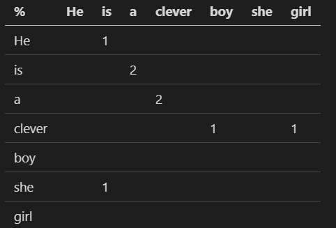
We can easily make the sliding window bigger and in both directions so for a central word “a” we have two words “is” and “clever” inside a sliding windows of size 1, and for the sliding window of size 2, the outside words (or contextual words for the word “a”) would be these four words:
- He
- is
- clever
- boy
If the text is big we can get big matrices, typically we could limit that to 10,000 words, because we can ignore words we don’t care about.
If we would like to deal with total 170,000 english words the matrix would be huge.
If we would slide just in one direction the matrix would not be symmetric. In numpy we could make it symmetric with this trick:
M = M + M.T
If we would like to get word projections in 2D or any kind of analysis we would need to lower the space so we need to use dimensionality reduction technique.
This would lower the dimension of our matrix from NxN to NxK where K<<N
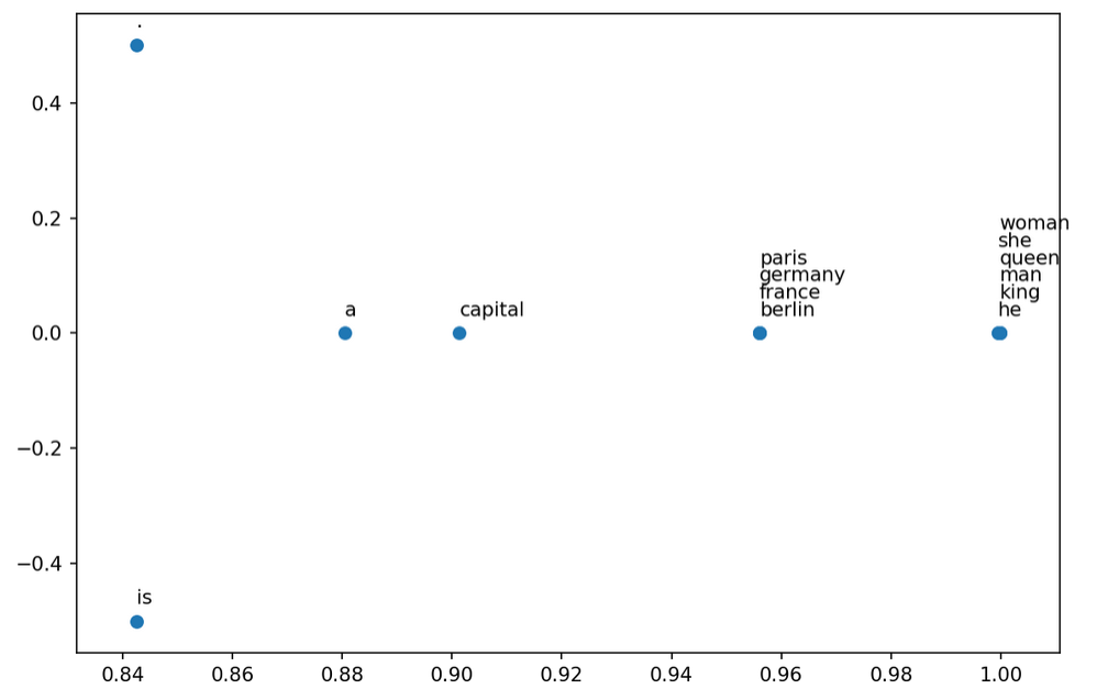
Example: Word representation in 2D space:
He is a king.
She is a queen.
He is a man.
She is a woman.
Berlin is germany capital.
Paris is france capital.
The next image shows the similar words:
word2vec
Then in 2013 one very important algorithm word2vec came along.
Using this algorithm it was possible to learn the representation of words where each word has 50 or more latent features.
The major gain with this latent approach–we are not forced to create co-occurrence matrices of NxN, where N is the number of distinct words. Instead all we have to learn is the NxK matrix where K is usually 100 (from 50 till 1000).
This break-trough idea published by Mikolov et al. was capable of doing word arithmetics for the first time:
W['king'] - W['man'] + W['woman'] = W['queen']
This provided a mean to deal with word analogies, because you could extend this idea to anything, but you could also understand the bias in a word model or the bias language in general may have.
The word2vec paper showed two new model algorithms called CBOW and skip-gram. CBOW is fast to train and skip-grap is more precise on majority of tasks they studied.
CBOW
CBOW introduced the average outside word:
$\begin{aligned} \large \boldsymbol{v} _ {a}=\frac{1}{2 h} \sum _ {n=1}^{k} \boldsymbol{v} _ {w _ {m+n}}+\boldsymbol{v} _ {w _ {m-n}} \end{aligned}$
- $k$ - window size, usually 4
- $\boldsymbol{v} _ {w}$ center word (embedding vector)
- $\boldsymbol{v} _ {w-k}, \cdots, \boldsymbol{v} _ {w-1}, \boldsymbol{v} _ {w+1}, \cdots, \boldsymbol{v} _ {w+k}$ context words as embedding vectors
$\begin{aligned} \log \mathrm{p}(\boldsymbol{w}) & \approx \sum _ {m=1}^{M} \log \mathrm{p}\left(w _ {m} \mid w _ {m-h}, w _ {m-h+1}, \ldots, w _ {m+h-1}, w _ {m+h}\right) \\ &=\sum _ {m=1}^{M} \log \frac{\exp \left(\boldsymbol{u} _ {w _ {m}} \cdot {\boldsymbol{v}} _ {a}\right)}{\sum_{j=1}^{V} \exp \left(\boldsymbol{u} _ {j} \cdot {\boldsymbol{v}} _ {a}\right)} \\ &=\sum _ {m=1}^{M} \boldsymbol{u} _ {w _ {m}} \cdot {\boldsymbol{v}} _ {a}-\log \sum _ {j=1}^{V} \exp \left(\boldsymbol{u} _ {j} \cdot {\boldsymbol{v}} _ {a}\right) \end{aligned}$
- $M$ - number of words in words lexicon
- $w _ {m}$ - center word at position $m$
- $\log \mathrm{p}(\boldsymbol{w})$ - entire corpus log likelihood
- $V$ - number of randomly sampled negative samples
Skip-gram
skip-gram is the other name for word2vec because this algorithm achieved best precision.
Essentially skip-gram uses logistic regression and answers the question what is the probability that neighbor word “blue” is near the central word “sky”.
$P(+ \mid C=”sky” , N=”blue”)$
(read: positive outcome that the central word “sky” has the neighbor/outside word “blue”)
The paper brought the notion of similarity using the dot product over the word embedding vectors.
$Similarity(C,N) = C \cdot N$
Similarity is not a probability, it can take values outside $[0,1]$ range. We could normalize it, but instead, even better, we fed similarity to logistic regression.
$\begin{aligned} P(+ \mid C,N) = \dfrac{1}{1+e^{C \cdot N}} \end{aligned}$
In skip-gram all outside words are conditionally independent so we can calculate the product of outside words for given central word:
$\begin{aligned} P(+ \mid \cdot) = P(+ \mid C, N _ i) \ \ \ i=1, \cdots , k \end{aligned}$
$\begin{aligned} P(+ \mid \cdot) = \prod _ {i=1}^k \dfrac{1}{1+e^{C \cdot N _ i }} \end{aligned}$
Since products are not numerically stable, we will switch to logs:
$\begin{aligned} \log P(+ \mid \cdot) = \sum _ {i=1}^{k} \log \dfrac{1}{1+e^{C \cdot N _ i}} \end{aligned}$
Similarly we can calculate entire corpus log likelihood:
$\begin{aligned} \log \mathrm{p}(\boldsymbol{w}) & \approx \sum _ {m=1}^{M} \sum _ {n=1}^{k _ {m}} \log \mathrm{p}\left(w _ {m-n} \mid w _ {m}\right)+\log \mathrm{p}\left(w _ {m+n} \mid w _ {m}\right) \\ &=\sum _ {m=1}^{M} \sum _ {n=1}^{k _ {m}} \log \frac{\exp \left(\boldsymbol{u} _ {w _ {m-n}} \cdot \boldsymbol{v} _ {w _ {m}}\right)}{\sum _ {j=1}^{V} \exp \left(\boldsymbol{u} _ {j} \cdot \boldsymbol{v} _ {w _ {m}}\right)}+\log \frac{\exp \left(\boldsymbol{u} _ {w _ {m+n}} \cdot \boldsymbol{v} _ {w _ {m}}\right)}{\sum _ {j=1}^{V} \exp \left(\boldsymbol{u} _ {j} \cdot \boldsymbol{v} _ {w _ {m}}\right)} \\ &=\sum _ {m=1}^{M} {\sum _ {n=1}^{k _ {m}} \boldsymbol{u} _ {w _ {m-n }} \cdot \boldsymbol{v} _ {w _ {m}}+\boldsymbol{u} _ {w _ {m+n}} \cdot \boldsymbol{v} _ {w _ {m}} -2 \operatorname {log} \sum _ {j=1}^{V} \operatorname {exp} ( \boldsymbol {u} _ {j}\cdot \boldsymbol{v} _ {w _ {m}})} \end{aligned}$
GloVe (Global Vectors)
GloVe paper was another direction in NLP.
It uses the context window and matrix factorization tricks like we would use for big co-occurrence matrices.
The difference is; instead of measuring word frequencies directly we take the log co-occurrence counts which improves the treatment of not so frequent words.
The paper also solved the problem when the co-occurrence count shouts over the maximal allowed number defined by the data format–in this case the number stays constant.
The Transformer model
In the 2017 the paper Attention Is All You Need changed the horizon of machine learning and NLP in general.
It introduced the attention to the NLP. The concept is based on vector dot product, parameters called Query, Key and Value and softmax function that learns the most probable combination of tokens. This was the advance from the models that learned the similarity of words.
It almost completely took the NLP world by storm, which at that time continuously made progress with LSTM, GRU and other recursive models–sequential in nature.
With models that are sequential in nature you convert words to tokens first and then you process tokens sequentially trough the model.
Transformer model processes the big number of tokens from once (512, 1024, or even greater) limited just with the amount of available memory and model size.
From the transformer model many new concepts started to grow. For instance, the famous BERT model would be the transformer where we removed the decoder part.
Nowadays, great attention is on GPT-2 and GPT-3 models and their modifications/extensions.
GPT based models can generate high quality text based on the initial inputs. These models can create newspaper articles or entire novels or they can generate HTML code based on some simple description or they can create Python code based on the function initial comments.
In general Transformers models can do all kind of NLP tasks.
Tokenizers
The key parts of the transformers are the so called tokenizers. Very popular tokenizers today are:
- Spacy
- WordPiece
- SentencePiece
- BPE
Here are models that use famous tokenizers:
- WordPiece: BERT, DistilBERT, Electra
- BPE: GPT-2, Roberta
- SentencePiece: T5, ALBERT, CamemBERT, XLMRoBERTa, XLNet, Marian
- Spacy: GPT
The great idea of custom tokenizer is that you can train the tokenizer to match your text corpora. Transformers library provides such tokenizers and training examples.
Great accent is on customizing transformer based models and achieving transfer learning and training the models from scratch, but you can use the already pretrained modes.
NLP libraries
There is a new Transformers library for NLP.
The little older NLP libraries you may use for many NLP tasks:
- nltk (Natural Language Toolkit)
- word2vec
- glove
- gensim
Example: Create tokens with nltk:
import nltk
nltk.download('punkt')

# import nltk.data
tokenizer = nltk.data.load('tokenizers/punkt/english.pickle')

from nltk.tokenize import word_tokenize

text = """He is a king.
She is a queen.
He is a man.
She is a woman.
Berlin is germany capital.
Paris is france capital."""
lists = nltk.tokenize.sent_tokenize(text)

short=[]
for sentence in lists:
    words= word_tokenize(sentence.lower())
    short.append(words)

pprint.pprint(short)
Output:
[['he', 'is', 'a', 'king', '.'],
 ['she', 'is', 'a', 'queen', '.'],
 ['he', 'is', 'a', 'man', '.'],
 ['she', 'is', 'a', 'woman', '.'],
 ['berlin', 'is', 'germany', 'capital', '.'],
 ['paris', 'is', 'france', 'capital', '.']]
Example: Find synonyms and hypenyms
import nltk
nltk.download('wordnet')
from nltk.corpus import wordnet as wn

# synonym set
for synset in wn.synsets('flush'):
    for l in synset.lemmas():
        print(l.name(), synset.pos() , synset)

# dog hypernyms
dog = wn.synset('dog.n.01')
list(dog.closure(lambda s: s.hypernyms()))
Output:
flower n Synset('flower.n.03')
prime n Synset('flower.n.03')
peak n Synset('flower.n.03')
heyday n Synset('flower.n.03')
bloom n Synset('flower.n.03')
blossom n Synset('flower.n.03')
efflorescence n Synset('flower.n.03')
flush n Synset('flower.n.03')
bloom n Synset('bloom.n.04')
blush n Synset('bloom.n.04')
flush n Synset('bloom.n.04')
rosiness n Synset('bloom.n.04')
hot_flash n Synset('hot_flash.n.01')
flush n Synset('hot_flash.n.01')
flush n Synset('flush.n.04')
bang n Synset('bang.n.04')
boot n Synset('bang.n.04')
charge n Synset('bang.n.04')
rush n Synset('bang.n.04')
flush n Synset('bang.n.04')
thrill n Synset('bang.n.04')
kick n Synset('bang.n.04')
flush n Synset('flush.n.06')
gush n Synset('flush.n.06')
outpouring n Synset('flush.n.06')
blush n Synset('blush.n.02')
flush n Synset('blush.n.02')
blush v Synset('blush.v.01')
crimson v Synset('blush.v.01')
flush v Synset('blush.v.01')
redden v Synset('blush.v.01')
flush v Synset('flush.v.02')
flush v Synset('flush.v.03')
flush v Synset('flush.v.04')
level v Synset('flush.v.04')
even_out v Synset('flush.v.04')
even v Synset('flush.v.04')
flush v Synset('flush.v.05')
scour v Synset('flush.v.05')
purge v Synset('flush.v.05')
sluice v Synset('sluice.v.02')
flush v Synset('sluice.v.02')
flush v Synset('flush.v.07')
flush s Synset('flush.s.01')
affluent s Synset('affluent.s.01')
flush s Synset('affluent.s.01')
loaded s Synset('affluent.s.01')
moneyed s Synset('affluent.s.01')
wealthy s Synset('affluent.s.01')
flush r Synset('flush.r.01')
flush r Synset('flush.r.02')


[Synset('canine.n.02'),
 Synset('domestic_animal.n.01'),
 Synset('carnivore.n.01'),
 Synset('animal.n.01'),
 Synset('placental.n.01'),
 Synset('organism.n.01'),
 Synset('mammal.n.01'),
 Synset('living_thing.n.01'),
 Synset('vertebrate.n.01'),
 Synset('whole.n.02'),
 Synset('chordate.n.01'),
 Synset('object.n.01'),
 Synset('physical_entity.n.01'),
 Synset('entity.n.01')]