ML brainstorming
- Types of machine learning
- Why do we have train, validation and test set
- What is overfitting?
- No Free Lunch Theorem
- Bias Variance tradeoff
- What is Cross-Validation (CV)
- CV when number of samples is small and lot of features
- Parametric vs. non-parametric models
- Generative vs. discriminative learning
- Convex and non-convex goal functions
- The two approaches to probability
- Bayesian approach
- Bayesian inference formula
- From Likelihood to cross entropy
- Binary cross entropy
- Multi-class classification
- What is a random variable
- Backpropagation (BP)
- Covariance
- Activation functions
- Error function
- Evaluation Metrics
- Linear models
- Regularization
- Optimizers
- General task of Machine Learning
- Nice Resources
Types of machine learning
Machine learning is usually divided into three main types:
- predictive or supervised learning
- descriptive (unsupervised) or self-supervised learning
- reinforcement learning
Predictive learning has the mapping from input $\mathbf x$ to output $y$.
Where $N$ is the number of training examples, $y_i$ is the single output feature, $\mathbf{x}_{i}$ is all the input features and $\mathcal{D}$ is the training set.
Descriptive learning doesn’t have a target.
It is sometimes called knowledge discovery and our goal is to find data patterns.
The problem with descriptive learning is there is no obvious error metric to use.
There is a mixture from the first two types called semi-supervised learning
Why do we have train, validation and test set
We need all three sets, train set to train, validation set to check if we are good.
We need some unseen data (test set) for our final check. If we would use the test set before, our machine learning parameters would be biased with the test data.
The purpose of the test set is to reflect some real data that we haven’t seen before.
What is overfitting?
If you train and test on the same data you make a methodological mistake.
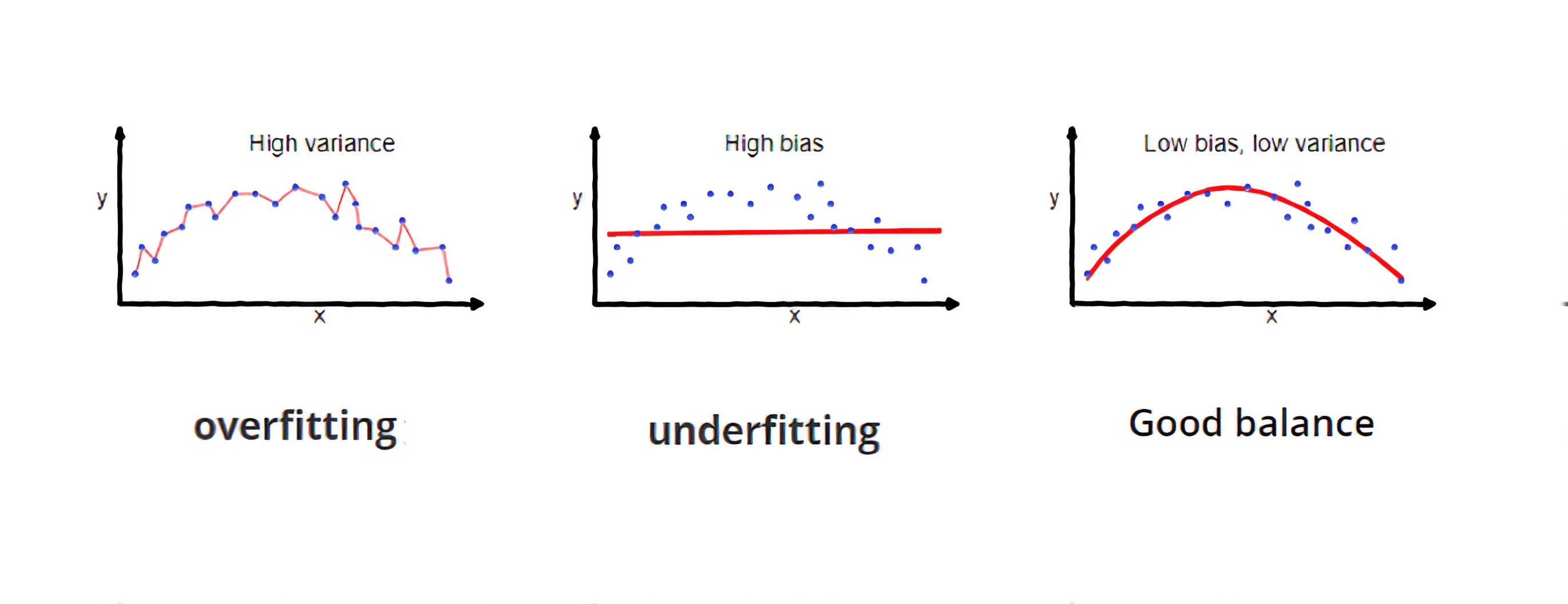
Overfitting is when the model learns the train data super well, and on unseen data it provides bad results.
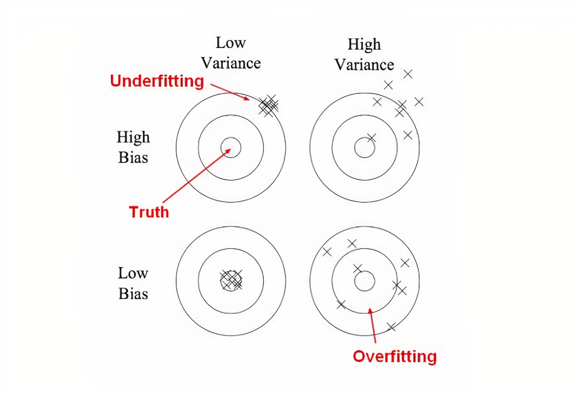
There is a big variance problem connected with overfitting while the bias is small.
Underfitting is a low variance and high bias problem.
No Free Lunch Theorem
According to “No Free Lunch Theorem” every successful machine learning algorithm must make assumptions about the model.
In other words there is no single machine learning algorithm that works best for all machine learning problems.
Bias Variance tradeoff
This is a simple fact, there is an optimal balance of bias and variance. It is where the total error is at the minimum.
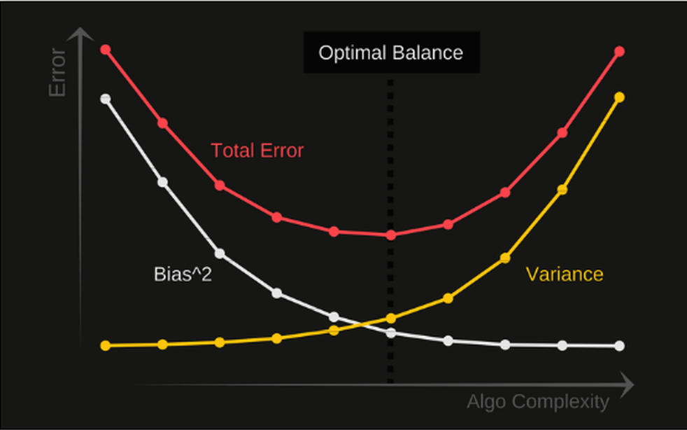
If we track the algorithm complexity there are two trends. The variance will increase with the increase of algorithm complexity.
The bias will decrease with the increase of the algorithm complexity.
The formula to calculate the total error is complex in general case, but if we use regression problem and MSE loss function the output should be:
Total Error = Bias^2 + Variance + Irreducible Error
Irreducible error is also called the noise, it is based on wrong labeling.
What is Cross-Validation (CV)
CV in the most basic form k-fold CV means the training set is split into k smaller sets.
In case of k-fold CV:
- the model is trained on
k-1folds as training data - the resulting model is validated on the remaining part of the data
CV when number of samples is small and lot of features
Say we have 5000 features and 50 samples to predict one of the two possible classes.
-
We could find top top 100 features (correlation)
-
We could then use CV on those 100 features and 50 samples.
But this would be a methodological mistake again. We should do a CV with all 5000 features instead.
Parametric vs. non-parametric models
There are two types of models:
- parametric
- non-parametric
In a parametric model, the number of parameters is fixed. In a nonparametric model the number of parameters can grow.
Some parametric models:
- The Perceptron
- Linear Regression
- Logistic Regression
- NB Naive Bayes
- Neural net with fixed architecture
The example of non-parametric machine learning models:
- KNN
- Decision trees
- Gaussian process
SVM (Support Vector Machines) can be both parametric and non-parametric.
Generative vs. discriminative learning
Discriminative algorithm given all measurements of a human will give you if the human is male or female.
Generative algorithms given a gender will generate a human.
Discriminative model focuses on what distinguishes the two or more classes.
A generative model models the distribution (detailed characteristics of each class).
SVM is an example of a discriminative model. NB is an example of a generative model.
Generative:
- KNN
- Naive Bayes
Discriminative:
- Decision trees
- Gaussian process
- Linear regression
- Logistic regression
Convex and non-convex goal functions
Support Vector Machines (SVM), Logistic Regression (LR) use convex goal functions. Neural Networks algorithms in general use non convex goal functions.
Semi-supervised problems in general lead to non-convex optimization problems, meaning the goal function is non convex.
The two approaches to probability
The basic fact about the probability it cannot be greater than 1 and lower than 0. For mathematicians the probability objective is to express how certain an event or statement is.
The so-called frequentists approach is to measure all possible outcomes of an event and to derive some conclusions about the event. For instance, rolling a regular (unbiased) or fair dice. The estimated probability to get 1 is $\tfrac{1}{6}$ that we got after 1 million measures.
The other approach is known as the Bayesian probability approach. For the same act rolling a fair dice, we may add some prior beliefs. We basically add our belief that we got 100 times 1, and then we start the measurements.
Else, if we don’t have any prior beliefs at all, this is called the uninformed prior.
Bayesian approach is especially important when we cannot do many measurements, or when the measurements are costly. For example, to answer the questions about how likely a person will catch a cold.
Bayesian approach
We often deal with uncertainty when we search for:
- the best prediction given data
- the best model given data
- what measurement should we perform next
The systematic application of probabilistic reasoning is called probabilistic approach or sometimes Bayesian approach.
Bayesian inference formula
In Bayesian inference we write the formula:
\[p(\theta|x)=p(\theta)L(\theta,x)c(x)\]where:
- $p(\theta)$ is the posterior
- $L(\theta,x)$ is the Likelihood
- $c(x)$ is a normalization constant
Probability vs. likelihood
Probability are the areas under the fixed distribution. In the image normal (continuous) distribution.
\[pr(data \mid \text{given parameters of normal distrubution $\mu$, $\sigma$})\]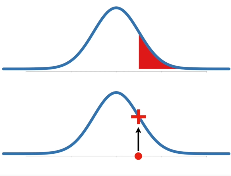
Likelihood are the fixed y-values for fixed x-point with distribution that can alter $\mu$, $\sigma$ distribution parameters.
\[L(\mu, \sigma \mid x=const)\]Likelihood must be at least 0, and can be greater than 1.
If we fix $x$, $\mu$ and $\theta$ we get the distribution function.
We can fix just $x$ and then we can check likelihood as a function of parameters $\theta$: $\mu$ and $\sigma$.
Example: Picking the candies from a box
Say we took the candies in this order:
Blue, Blue, Red, Red, Blue. This is our training set.
Empirical probability of red in the training set would be $p_{red}={2\over5}$ $p_{blue}={3\over5}$.
If we guess probabilities in two ways; with a bad and with a good model:
$q_{red}^{bad}={4\over5}$ $q_{blue}^{bad}={1\over5}$
$q_{red}^{good}={2.5\over5}$ $q_{blue}^{good}={2.5\over5}$
How would the bad model describe the training set?
$L(q^{bad}) = ({4 \over 5})^2({1 \over 5})^3={16\over25}{1\over125} = 0.00512$
How would the good model describe the training set using the likelihood function?
$L(q^{good}) = {1 \over 32} = 0.03125$
How would the perfect model describe the training set?
$L(q^{perfect}) = ({2 \over 5})^2({3 \over 5})^3=0.03456$
From Likelihood to cross entropy
In previous example the likelihood of the training set would be proportional to:
\[\prod_i {q_i}^{Np_i}\]We convert likelihood to log likelihood:
\[{1\over {N}} \text {log} \prod_i {q_i}^{Np_i} = \sum_i p_i \text {log}(q_i) =-H(p,q)\]This log likelihood is cross entropy.
Binary cross entropy
For the binary case we may have the binary cross entropy:
\[H(p,q) = - \sum_i p_i \text {log}(q_i) =-y \text{log}(\hat y)-(1-y)\text{log}(1-\hat y)\]$p_i$ and $q_i$ are probabilities of outcome in the training set, and estimated probability of outcome.
Where the entropy is minimized the likelihood is maximized and the model is expressive.
Multi-class classification
If the number of classes >2 we use the multi-class classification with softmax.
Softmax function will normalize the sum of output probabilities to 1. The target or the ground truth class will have the $\hat y=1$, else 0.
The cross entropy loss formula will be a big sum:
\[L_{ce}=-\sum_i y_i \text{log}(\hat y_i)\]The smaller the loss the better the model predicts.
What is a random variable
As it turns out, the idea of a random variable (also called stochastic) is very important when dealing with probabilities. Random variables can be discrete and continuous.
A finite collection of random variables defined under certain conditions is a random vector.
An infinite collection of random variables defined under certain conditions is a random process.
A latent variable is a random variable that we cannot observe directly.
A proper formal understanding of random variables is defined via a branch of mathematics known as measure theory. Measure theory defines terms such as:
- almost everywhere
- measure zero set
In short: A random variable is a variable whose possible values have an associated probability distribution.
Check more on probability distributions
How you estimate the distribution from the data
This is one of the main questions in machine learning (probabilistic approach)
There are few ways to estimate distributions from data:
- MLE (Maximum Likelihood Estimation)
- MAP (Maximum A Posteriori Estimation)
- Bayesian inference
For MLE if we have to maximize $P(\mathcal D \mid \theta)$, where $\theta$ is a set of parameters,
For MAP we have $P(\theta \mid \mathcal D)$, where $\theta$ is a random variable now.
$\theta$ need to be random variable so we can use the Bayes rule:
$P(\theta \mid \mathcal D) = \large \frac{P(\mathcal D \mid \theta )P(\theta)}{z}$, where $z$ is normalization constant.
In both cases we end with the pattern $P(\mathcal D \mid \theta )$ to maximize which means MLE and MAP will have similar algorithmic steps.
Bayesian inference returns probability density function and is complex to calculate.
$P(y_{t} \mid \mathbf x_{t}) = \int_{\theta} P(y_{t} \mid \mathbf x_{t} , \theta) P(\theta \mid \mathcal D) d\theta$
To calculate this integral is hard and this is why in practice we use pragmatic MLE and MAP approaches.
What is the difference: MLE and MAP
MAP is a pragmatic approach to Bayesian optimization where we take say thousand different $\theta$s and we average those.
It’s like systematically trying different parameters and defining what are the best parameters. If we have just two parameters imagine creating a grid with different values for all the parameters and finding the best parameters.
MLE gives the value which maximizes the likelihood $P(\mathcal D \mid \theta)$. And MAP gives you the value which maximizes the posterior probability $P(\theta \mid \mathcal D)$.
Backpropagation (BP)
BP is the process of calculating the derivatives.
Gradient Descent (GD)
Once we have the derivatives and gradient descent is the process of descending through the gradient and adjusting the parameters of the model through the error function.
GD is a first-order Taylor expansion iterative optimization algorithm for finding a local minimum of a differentiable function using the learning rate.
Newton method
Second order Taylor expansion would be the Newton method.
Newton’s method is used for maximization/minimization of a function using knowledge of its second derivative.
It has stronger constraints in terms of the differentiability of the function than gradient descent.
If the second derivative of the function is undefined in the function’s root, Newton’s method won’t work.
Newton’s method has fast convergence (in just a few steps) to the local minima.
Constraints of the Newton method:
- the Newton method may not converge (no luck)
- If the dimensionality of the data is huge it is hard to compute the Hessian ($D^2$), and inverse of Hessian ($D^3$), Where $D$ is the dimensionality of the data.
Note the dataset may have large number of features $f$ and large number of data samples $n$, but the dimensionality of the data may just be $D=10$
In case we use the diagonal of a Hessian, we can approximate Newton’s method. This way it is easy to compute the Hessian even for large values of $D$.
Gradient Descent vs. Newton method
If we use Taylor expansion linear approximation we are in the domain of gradient descent.
GD is an iterative optimization algorithm for finding a local minimum of a differentiable function.
If we use second order Taylor expansion we are in the domain of Newton method.
Gradient Descent (GD) vs. Stochastic Gradient Descent (SGD)
If we perform forward pass using ALL the train data before backpropagation pass to adjust the weights this is called GD.
One step of GD is one one epoch.
In SGD we perform the forward pass using a SUBSET of the train data. These subsets are called mini-batches.
Target Propagation
The main idea of target propagation is to compute targets rather than gradients, at each layer. Target propagation relies on auto-encoders at each layer.
Covariance
Covariance means linear dependence between two random variables.
Activation functions
The most important features of the activation functions are:
- function input range
- function output range
- if the function is monotonic
- number of kinks
- what is the derivative of a function
- if derivative is monotonic
Some activation functions:
- Sigmoid
- Tanh
- Leaky ReLU
- ReLU
- SoftPlus (differentiable version of ReLU)
- CELU (continuously differentiable Exponential Linear Unit)
Why ReLU is better than Sigmoid activation function
This reflects the fact that the brain (dendrons) use ReLU. Dendrons fire the axon if a certain condition is achieved. Usually things work better when we imitate nature.
The formally accepted reason why ReLU is better than sigmoid is related to the vanishing gradient problem. There are no such problems for ReLU or modifications while Sigmoids suffers from this problem for input greater than 6 in absolute value.
Also, ReLu is faster to compute than the sigmoid function, and its derivative is faster to compute.
The problem with ReLU, it is not a smooth function near $x=0$.
Error function
Objective function or criterion is the function we want to minimize or maximize.
A loss function is for a single training example.
A cost function is the average loss over the entire training dataset.
Error function is a generic term for both loss and cost function.
Error function vs. evaluation metrics
Error function that will get minimized by the optimizer.
An evaluation metric is used to check the performance of the model. Evaluation metrics are used to check the model quality and it is not related to the optimization process.
Error function and evaluation metrics may not be the same.
Evaluation Metrics
An evaluation metric checks the performance of a model.
There are different metrics for the tasks of classification, regression, ranking, clustering, topic modeling, etc.
It is very important to use multiple evaluation metrics to evaluate your model.
Regression metrics
- MSE Mean Squared Error
- RMSE Root Mean Squared Error
- MAE Mean Absolute Error
- MAPE Mean Absolute Percentage Error
- MSLE Mean Squared Logarithmic Error
- Cosine Similarity
- LogCoshError
The mathematical reasoning behind the MSE is as follows: For any real applications, noise in the readings or the labels is inevitable.
We generally assume this noise follows Gaussian distribution and this holds perfectly well for most of the real applications. Considering $e$ follows a Gaussian distribution in $y=f(x) + e$ and calculating the MLE, we get MSE which is also L2 distance.
Assuming some other noise distribution may lead to other MLE estimates which will not be MSE.
Classification metrics
- Accuracy
- Logarithmic Loss
- Confusion Matrix
- Precision
- Recall
- and F-score
- ROC/AUC
Classification accuracy is the ratio of the number of correct predictions to the total number of input samples
Logarithmic loss, also called log loss, works by penalizing the false classifications.
A confusion matrix gives us a matrix as output and describes the complete performance of the model.
$P = TP/ (TP+FP)$
$R = TP / (TP+FN)$
$F_1 = 2PR/(P+R)$
$F_{\beta}=(1+\beta^{2}) PR / (\beta^{2} P + R )$
Linear models
Well known linear models are linear regression and logistic regression.
Both these algorithms are based on supervised learning.
Linear Regression
There are different types of linear regression:
- Simple linear regression: models using only one predictor
- Multiple linear regression: models using multiple predictors
- Multivariate linear regression: models for multiple response variables
There is also a generalized linear model as generalization of linear regression that allows for the response variable to have an error distribution other than the normal distribution.
Linear regression has a closed form solution meaning that the algorithm can get the optimal parameters by just using a formula that includes a few matrix multiplications and inversions.
Logistic Regression
Logistic regression uses a sigmoid function which transforms output and returns regular probability value from 0 to 1.
This output value will be mapped to two or more classes.
If two classes of output we represent this with: $y={0,1}$ and call it binary logistic regression.
The cost function of logistic regression is log loss or Cross-Entropy loss.
If we have more than 2 output classes this is called multiclass logistic regression.
Output is then: $y={0,1, … , n }$
We re-run binary classification multiple times, once for each class.
If we have $n$ classes we divide the problem into $n$ binary classification problems.
Often we need to work with a special version of sigmoid function called softmax or softargmax function.
This softargmax will apply the standard exponential function to each element of the input vector and normalize these values by dividing by the sum of all these exponentials. The sum of all output vectors will add to 1.
The sigmoid, or softmax function outputs a probability, whereas the inverse Logit function takes a probability and produces a real number.
Loss function is sum of cost functions:
\[\begin{array}{ll} J(\theta)=\frac{1}{m} \sum_{i=1}^{m} \operatorname{Cost}\left(h_{\theta}\left(x^{(i)}\right), y^{(i)}\right) & \\ \operatorname{Cost}\left(h_{\theta}(x), y\right)=-\log \left(h_{\theta}(x)\right) & \text { if } \mathrm{y}=1 \\ \operatorname{Cost}\left(h_{\theta}(x), y\right)=-\log \left(1-h_{\theta}(x)\right) & \text { if } \mathrm{y}=0 \end{array}\]Cost functions differ for $y=1$ and $y=0$.
Jacobian vs. Hessian
The Jacobian is then the generalization of the gradient for vector-valued functions of several variables.
Hessian Matrix is a square matrix of second-order partial derivatives of a scalar-valued function, or scalar field. It describes the local curvature of a function of many variables.
Regularization
The general idea of regularization is to eliminate the overfitting. Several options in there:
Adding noise
Adding noise is only during the training.
With noise the model is not able to memorize training samples because they are changing resulting in network low generalization error.
Noise can be added either on weights or on the output. When adding the noise in the output we call it label smoothing.
Ensembling
Either bagging, boosting or stacking.
In the case of decision trees that would be the random forest. A large number of relatively strong learners in parallel.
Strong learners combined will provide the solution that minimizes the variance of individuals.
Boosting combines weak learners into strong learners. It works like a swarm of bees. Individual bees are unsure of the exact place for the beehive, but together they find an ideal place. The principle minimizes the individual bias.
Stacking combines different algorithm types and creates multi level architecture that will at the end improve the bias and the variance of individual solutions.
In all ensemble methods different strong/weak learners are fitted independently from each other.
Early stopping
Possible after $e$ epochs the model will start with overfitting since the training data are well learned.
Early stopping is a technique to stop after some number of epochs once the evaluation metrics start to show the increase of the error.
L1 and L2 regularization
Difference based on how the loss is calculated:
$L_1 = Error(Y - \widehat{Y}) + \lambda \sum_1^n \mid w_i \mid$
$L_2 = Error(Y - \widehat{Y}) + \lambda \sum_1^n w_i^{2}$
L1 regularization tries to estimate the median of the data while the L2 regularization tries to estimate the mean of the data to avoid overfitting.
Use L1 or Lasso regularization if you have a great number of weights to shrink them to 0.
This way we can use L1 for feature selection, as we can drop any variables associated with coefficients that go to zero.
Use L2 or Ridge regularization will penalize weights evenly. L2 is useful when you have collinear features.
L1, L2 are also known as Weight Decay
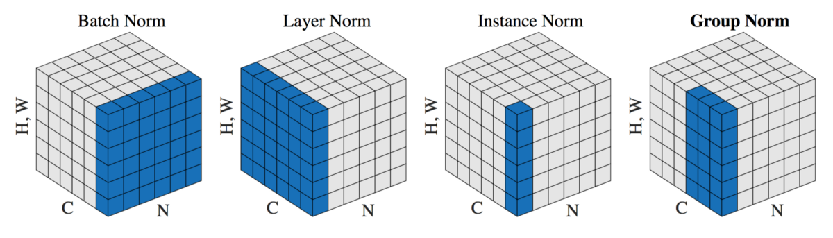
Batch Norm
BN resets the distribution of the previous layer and transmits to the next layer for efficient processing.
After BN all activation values are normalized $\mathcal N(0, 1)$.
BN ensures bigger learning rates can be used.
BN adds two additional trainable parameters:
- the normalized output that’s multiplied by standard deviation (gamma parameter)
- and the additional mean (beta parameter)
This way we say batch normalization works together with gradient descents.
Whitening version of Batch Norm
Batch norm does a good job at controlling distributions of individual channels, but doesn’t tackle covariance between channels.
Whitening version of the batch norm will do ZCA to remove input correlations.
Other norms
There is no universal normalization method that can solve all application problems.
Other norms are Layer norm especially used in the transformer architecture.
Instance norm normalizes each element of the batch independently across spatial locations only and for all the channels.
Other regularization options
Other regularization options include:
- regularization based on optimization function
- regularization based on error function
- data based regularization such as: large batch size, half precision, cross validation, using different activation functions, test-time augmentation, …
Optimizers
- GD (Not practical because it performs computations on the whole dataset)
- SGD (only computes a mini-batch of data examples)
- Adam (the best among the adaptive optimizers in most of the cases and good with sparse data, has the adaptive learning rate)
- AdaGrad (has no momentum, uses different learning rates for each dimension)
General task of Machine Learning
The general task in ML is to reduce Entropy.
Entropy is a measure of chaos or uncertainty. The goal of machine learning models is to reduce this uncertainty.
The lower the entropy the more information is gained about the target from the features.
Nice Resources
Great resources to learn ML in 2021 are: