Logistic Regression
Logistic regression is a classification algorithm. It assumes that the response variable only takes on two possible outcomes.
LR is a supervised method
The following diagram describes the general supervised model:
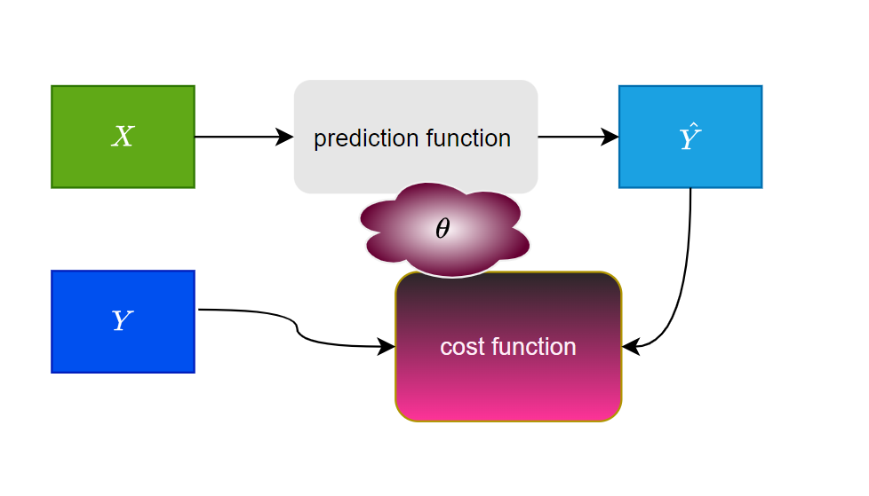
- $X$ are the input features.
- $Y$ are labels
- $\hat Y$ would be the output after the prediction.
- $\theta$ are the parameters we update.
- The cost function is used to compare the original labels $Y$ and the predicted labels.
- For Logistic Regression the Sigmoid prediction function is used.
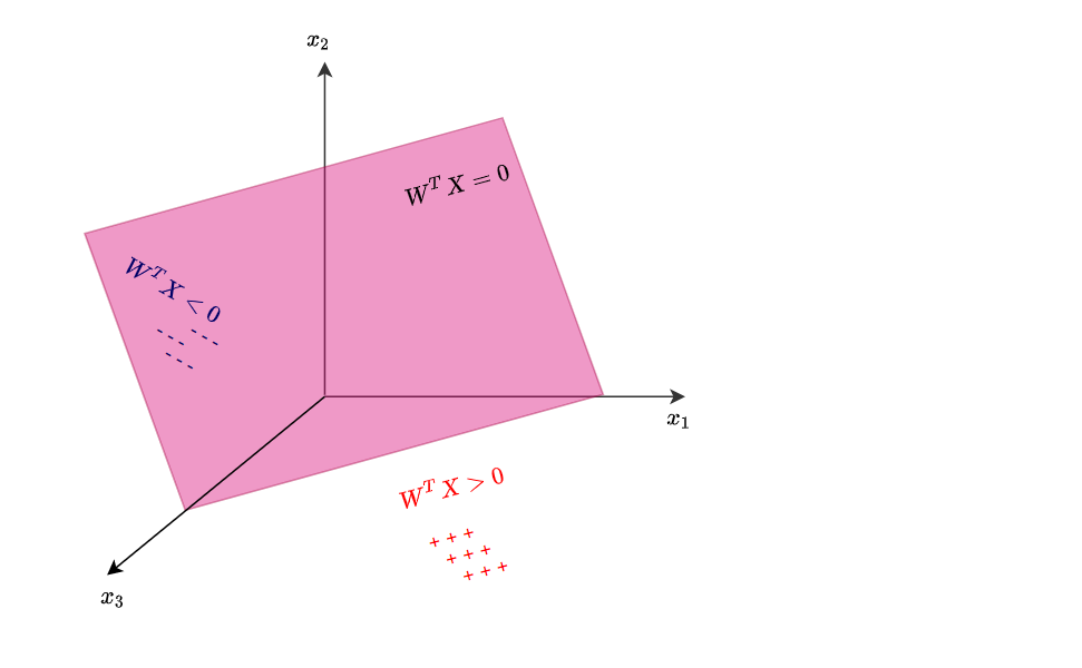
Positive or negative classification
We are able to define the line $W^TX=0$.
Vector notation can be written: $W^TX=w_0x_0+w_1x_1+\ … + w_dx_d$. Where $d$ is the dimension of input features, and $w_0$ is bias and $x_0$ is set to 1 (not to worry about this detail).
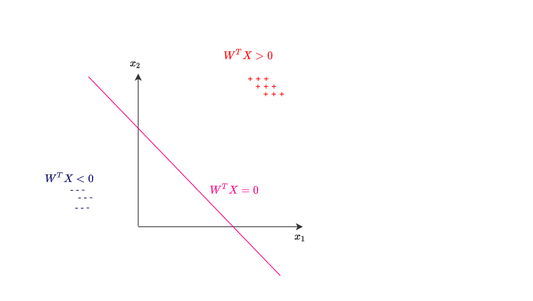
We define two classes $W^TX>0$ (positive) and $W^TX<0$ (negative).
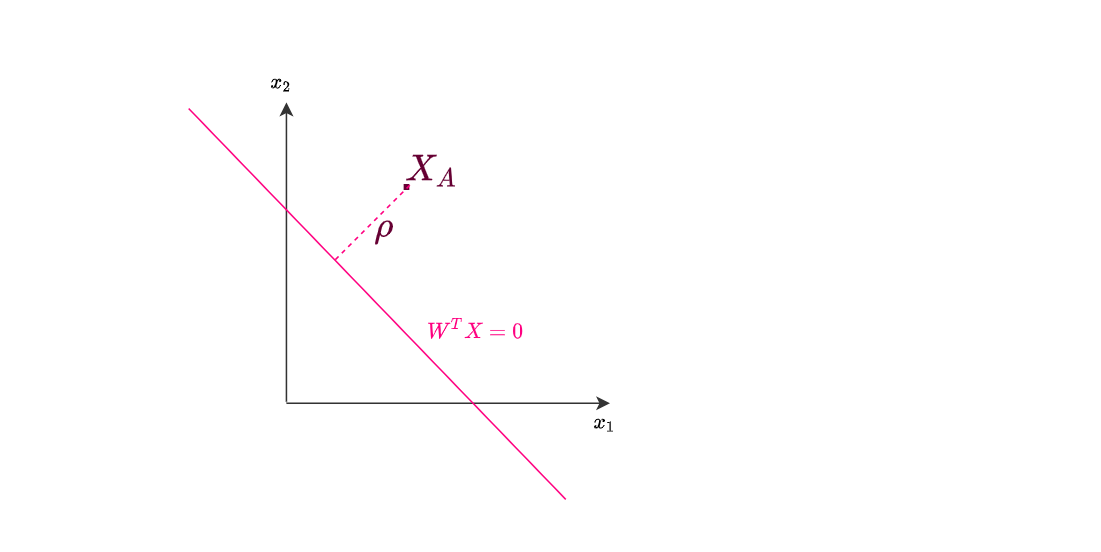
We can also define the point $X_A$ whose distance from the pink line (hyperplane) is $\rho$:
\[\rho = \frac{W^TX }{\|W \|_2}\]This way the $\texttt{sign}(\rho)$ indicates if the example is positive or negative. In the image the point $X_A$ is a positive example, because the $\rho >0$.
In general binary classification can go to either positive or negative class:
\[\texttt{sign}(\rho) \in \{-1, 1\}\]To calculate the L2 norm you use:
\[\| {W} \|_2 = \sqrt{\sum_{i=0}^d w_i^2}\]where $d$ is the dimension of the hyperplane and for $w_0$ represents the bias and is usually set to 1.
LR probabilities
It is not sufficient to just find the class, but also to provide the info about the positive prediction.
How can we map $W^TX$ into $[0,1]$ probability space?
If the $\rho=0$ we cannot say which class we have. If $\rho$ is infinitely large the probability should be 1. Same for infinitely small. In between the probability should be smaller than 1.
\(\hat {P}_{+} = P \{ y=+1 \mid X \} \in [0,1]\)
\(\hat {P}_{-} = P \{ y=-1 \mid X \} \in [0,1]\)
We can make odds ratio:
$\frac{\hat P_{+}}{\hat P_{-}}\in [0, +\inf)$
Then: $\texttt{log}\frac{\hat P_{+}}{\hat P_{-}} = W^TX$
Logistic regression predicts probability $\hat P_{+}$ as: \(\hat P_{+}=\frac{1}{1+e^{-W^TX}}=\texttt{sigmoid}(W^TX)\)
LR is discriminative model
LR is a discriminative model because it has a hyperplane between the two classes.
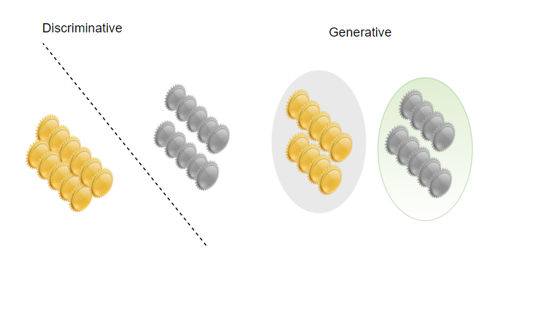
In discriminative approach we fit a model of the $p(Y \mid X)$ posterior directly.
Binary classification model
$P(Y \mid X, W)=\texttt{Ber}\left(Y \mid \texttt{sigm}\left(W^{T} X\right)\right)$
$P$ denotes discrete distribution, $p$ continuous, $\operatorname{sigm}$ is sigmoid function.
Logistic Regression is linear model
A classifier is linear if its decision boundary on the feature space is a linear function: positive and negative examples are separated by a hyperplane.
Logistic regression outcome depends on the sum of the input features and parameters. The output cannot depend on the product of features, or the features are independent of each other.
Logistic regression uses linear decision boundaries. Imagine you trained a logistic regression and obtained the coefficients $w_i$. You might want to classify a test record if $P(x) > 0.5$, where $x_{i} \in \mathbb{R}^{d}$.
The probability is obtained with your logistic regression by: \(P(x) = \frac{1}{1+e^{-(w_0 + w_1 x_1 + \dots + w_d x_d)}}\)
If you work out the math you see that $P({x}) > 0.5$ defines a hyperplane on the feature space which separates positive from negative examples.
Logloss
$\texttt {logloss}(x_i, y_i) = log(1+e^{-y_iW^TX_i})$
where
\(y_i\in\{-1, +1\}\)
In here, part: $y_iW^TX_i$ is called margin $M$.
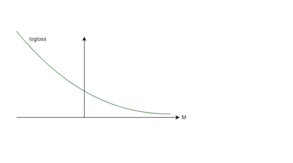
Logloss is differentiable and monotonous. From this reason we can use this function to calculate parameters $w_i$ in optimization procedure.
If we would have loss function that is differentiable, but not monotonous we couldn’t use it for LR.
Any differentiable function would still work for gradient boosting.
LR model
To model LR we take $m$ samples $ {x_{i}, y_{i}} $ such that $x_{i} \in \mathbb{R}^{d}$ and $y_{i} \in \mathbb{R}$.
In here $y_i$ is our dependent variable and $x_i$ is independent variable. You can consider $x_i$ are multiple columns, while $y_i$ is the target column.
$d$ is how many independent columns we have.
To define the formal model we need:
- hypothesis function,
- loss function
You may guess hypothesis function is the logistic function (also known as: logit, sigmoid, $\sigma$)
$ h_{\theta}\left(x_{i}\right)=\sigma\left(\omega^{T} x_{i}\right)=\sigma\left(z_{i}\right)=\frac{1}{1+e^{-z_{i}}} $
Where $\omega \in \mathbb{R}^{d}$ and $z_{i}=\omega^{T} x_{i} .$
We will be computing gradients in here w.r.t. weights $\omega$
The loss function is then defined as: \(l(\omega)=\sum_{i=1}^{m}-\left(y_{i} \log \sigma\left(z_{i}\right)+\left(1-y_{i}\right) \log \left(1-\sigma\left(z_{i}\right)\right)\right)\)
Or in indexed notation: \(l_i(\omega)=-y_i\log\sigma(z_i)-(1-y_i)\log(1-\sigma(z_i))\)
Utilizing some properties of logistic function
Derivation property :
$\frac{d}{d z} \sigma(z)= \frac{d}{d z}\left(\frac{1}{1+e^{-z}}\right)=-\frac{-e^{-z}}{\left(1+e^{-z}\right)^{2}}=\frac{1}{1+e^{-z}} \cdot \frac{e^{-z}}{1+e^{-z}}=\sigma(z)(1-\sigma(z))$
Negative property :
$\sigma(-z) =1 /\left(1+e^{z}\right) =e^{-z} /\left(1+e^{-z}\right) =1-1 /\left(1+e^{-z}\right)= 1-\sigma(z)$
We will also need to express $x$ and $x^T$ in terms of $z$:
$\frac{\partial z}{\partial \omega}=\frac{x^{T} \omega}{\partial \omega}=x^{T}$
$\frac{\partial z}{\partial \omega^{T}}=\frac{\partial \omega^{T} x}{\partial \omega^{T}}=x$
Computing Gradient and Hessian
- Gradient $\nabla_{\omega} l(\omega)$
- Hessian $\nabla_{\omega}^2 l(\omega)$
We start from indexed notation of the loss:
\(l_i(\omega)=-y_i\log\sigma(z_i)-(1-y_i)\log(1-\sigma(z_i))\) and we will first express the $\log\sigma(z_i)$ and $\log(1-\sigma(z_i))$.
…
\[\begin{aligned} \frac{\partial \log \sigma\left(z_{i}\right)}{\partial \omega^{T}} &=\frac{1}{\sigma\left(z_{i}\right)} \frac{\partial \sigma\left(z_{i}\right)}{\partial \omega^{T}}=\frac{1}{\sigma\left(z_{i}\right)} \frac{\partial \sigma\left(z_{i}\right)}{\partial z_{i}} \frac{\partial z_{i}}{\partial \omega^{T}}=\left(1-\sigma\left(z_{i}\right)\right) x_{i} \\ \frac{\partial \log \left(1-\sigma\left(z_{i}\right)\right)}{\partial \omega^{T}} &=\frac{1}{1-\sigma\left(z_{i}\right)} \frac{\partial\left(1-\sigma\left(z_{i}\right)\right)}{\partial \omega^{T}}=-\sigma\left(z_{i}\right) x_{i} \end{aligned}\]Finally
\[\nabla_{\omega} l_{i}(\omega)=\frac{\partial l_{i}(\omega)}{\partial \omega^{T}}=-y_{i} x_{i}\left(1-\sigma\left(z_{i}\right)\right)+\left(1-y_{i}\right) x_{i} \sigma\left(z_{i}\right)=x_{i}\left(\sigma\left(z_{i}\right)-y_{i}\right)\]And in vector notation :
$\nabla_{\omega} l_{i}(\omega)=\sum_{i}\left(\mu_{i}-y_{i}\right) \boldsymbol{x}_{i}$
Now to compute the Hessian:
\(\nabla_{\omega}^{2} l_{i}(\omega)=\frac{\partial l_{i}(\omega)}{\partial \omega \partial \omega^{T}}=x_{i} x_{i}^{T} \sigma\left(z_{i}\right)\left(1-\sigma\left(z_{i}\right)\right)\) For $m$ samples we have ${\nabla_{\omega}}^{2} l(\omega)=\sum_{i=1}^{m} x_{i} x_{i}^{T} \sigma\left(z_{i}\right)\left(1-\sigma\left(z_{i}\right)\right)$.
This is equivalent to concatenating column vectors $x_{i} \in \mathbb{R}^{d}$ into a matrix $X$ of size $d \times m$ such that
\[\sum_{i=1}^{m} x_{i} x_{i}^{T}=X X^{T}\]The scaling terms are combined in a diagonal matrix $S$ such that $S_{i i}=\sigma\left(z_{i}\right)\left(1-\sigma\left(z_{i}\right)\right)$.
Finally, Hessian w.r.t. weights of the loss function is: \({H}(\omega)=\nabla_{\omega}^{2} l(\omega)=X S X^{T}\)