KL Divergence | Relative Entropy
- Terminology
- What is KL divergence really
- KL divergence properties
- KL intuition building
- OVL of two univariate Gaussian
- Express KL divergence via Cross Entropy minus Entropy
- Machine learning application
- KL as a distance metric
- Conclusion
Terminology
Kullback-Leibler Divergence (KL Divergence) known in statistics and mathematics is the same as relative entropy in machine learning and Python Scipy.
Let’s start with the Python implementation to calculate the relative entropy of two lists:
p=[0.2, 0.3, 0.5]
q=[0.1, 0.6, 0.3]

def kl(a, b):
    '''
    numpy formula to calculate the KL divergence

    Parameters:
      a: probability distribution of RV X
      b: another probability distribution of RV X
    Output:
      kl score always positive, or 0 in case a=b
    '''
    a = np.asarray(a, dtype=np.float)
    b = np.asarray(b, dtype=np.float)
    return np.sum(np.where(a != 0, a * np.log(a / b), 0))
k = kl(p,q)
print(k)
Output:
0.18609809382700082
What is KL divergence really
We start by referring the basics:
Probability should add to 1
$\begin{aligned}\int_{-\infty}^{\infty} p(x) \mathrm{d} x =1\end{aligned}$
Expected value of the distribution $p$:
$\begin{aligned}\mu = \int_{-\infty}^{\infty} x p(x) \mathrm{d} x \end{aligned}$
Variation formula, uses the expected value $\mu$.
$\begin{aligned}\sigma^{2} =\int_{-\infty}^{\infty}(x-\mu)^{2} p(x) \mathrm{d} x \end{aligned}$
KL divergence answers the question how different are two probability distributions $p$ and $q$ at any point $x$.
$\begin{aligned}D_{KL} (q \parallel p)=\int_{-\infty}^{\infty} q(x) \log \frac{q(x)}{p(x)} d x\end{aligned}$
Recall that the $q(x)$ and $p(x)$ are probabilities and that the Shannon information is defined as:
$I(x) = -\log_2 q(x)$
This means KL is the expected value of information ratio.
$\begin{aligned}D_{KL}(q \parallel p) = - \mathbb{E}_{q}\left[-\log \frac{q}{p}\right]\end{aligned}$
KL divergence properties
The last property is easy to prove thanks to Jensen’s inequality for concave functions and logarithm is a concave function.
The function is concave if its second derivative is negative
KL intuition building
Now let’s compare KL divergence of two Gaussian distributions:
$f(x)=\Large \frac{1}{\sqrt{2 \pi \sigma^{2}}} e^{-\frac{(x-\mu)^{2}}{2 \sigma^{2}}}$
I like to use formulas with $\sigma^2$, because it’s inverse to precision $\gamma$.
We made a Python program to draw this PDF.
%matplotlib inline
import numpy as np
from matplotlib import pyplot as plt
plt.rcParams['figure.dpi'] = 100

def gaussian_pdf(mu, sigma, x):
    '''
    Gaussian pdf
    Parameters:
        mu: mean
        sigma: standard deviation
    Output:
        calculated PDF value
    '''

    'coefficient'
    c = 1/(np.sqrt(2*math.pi*sigma**2))
    'exponent'
    e = ((x-mu)**2/2*sigma**2)

    return c*np.exp(e)

gaussian_pdf(0,1,0)
# 0.3989422804014327
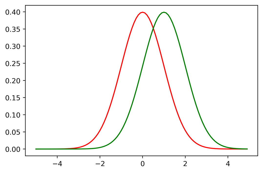
First plot:
x = np.arange(-5., 5., 0.1)
plt.plot(x,gaussian_pdf(0,1,x),color='r') # mu=0, sigma=1
plt.plot(x,gaussian_pdf(1,1,x),color='g') # mu=1, sigma=1
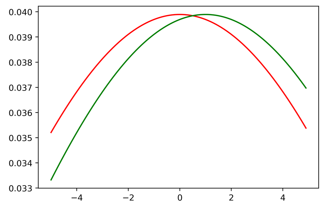
Second plot:
x = np.arange(-5., 5., 0.1)
plt.plot(x,gaussian_pdf(0,10,x),color='r') # mu=0, sigma=10
plt.plot(x,gaussian_pdf(1,10,x),color='g') # mu=1, sigma=10
To compute the KL divergence between two Gaussian univariate functions we have the formula:
\[\begin{aligned} D_{KL}(p \parallel q) &=-\int p(x) \log q(x) d x+\int p(x) \log p(x) d x \\ &=\frac{1}{2} \log \left(2 \pi \sigma_{2}^{2}\right)+\frac{\sigma_{1}^{2}+\left(\mu_{1}-\mu_{2}\right)^{2}}{2 \sigma_{2}^{2}}-\frac{1}{2}\left(1+\log 2 \pi \sigma_{1}^{2}\right) \\ &=\log \frac{\sigma_{2}}{\sigma_{1}}+\frac{\sigma_{1}^{2}+\left(\mu_{1}-\mu_{2}\right)^{2}}{2 \sigma_{2}^{2}}-\frac{1}{2} \end{aligned}\]Calculation:
In the first case: $\mathcal N(0,1)$ and $\mathcal N(1,1)$
$D_{KL}(p\parallel q)=0.5$
Second case: $\mathcal N(0,10)$ and $\mathcal N(1,10)$
$D_{KL}(p\parallel q)=0.005$
Note in the second case the divergence is smaller.
OVL of two univariate Gaussian
We are building our KL divergence intuition further.
If we create a program in R to solve the OVL (overlapping coefficient) of the two Gaussian PDFs:
min.f1f2 <- function(x, mu1, mu2, sd1, sd2) {
    f1 <- dnorm(x, mean=mu1, sd=sd1)
    f2 <- dnorm(x, mean=mu2, sd=sd2)
    pmin(f1, f2)
}

mu1 <- 0;    sd1 <- 1
mu2 <- 1;    sd2 <- 1

xs <- seq(min(mu1 - 3*sd1, mu2 - 3*sd2), max(mu1 + 3*sd1, mu2 + 3*sd2), .01)
f1 <- dnorm(xs, mean=mu1, sd=sd1)
f2 <- dnorm(xs, mean=mu2, sd=sd2)

plot(xs, f1, type="l", ylim=c(0, max(f1,f2)), ylab="density")
lines(xs, f2, lty="dotted")
ys <- min.f1f2(xs, mu1=mu1, mu2=mu2, sd1=sd1, sd2=sd2)
xs <- c(xs, xs[1])
ys <- c(ys, ys[1])
polygon(xs, ys, col="gray")

### only works for sd1 = sd2
SMD <- (mu1-mu2)/sd1
2 * pnorm(-abs(SMD)/2)

### this works in general
integrate(min.f1f2, -Inf, Inf, mu1=mu1, mu2=mu2, sd1=sd1, sd2=sd2)
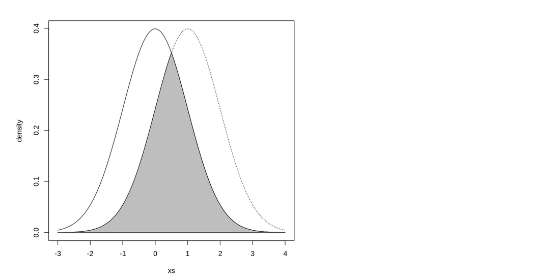
In here the OVL coefficient will be 0.617
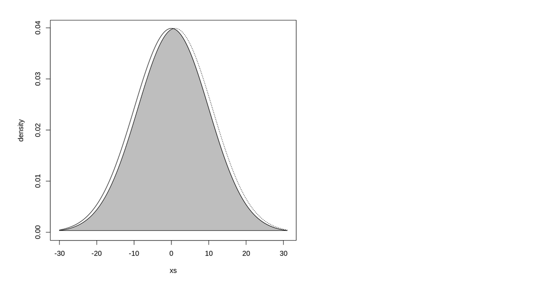
In here the OVL coefficient will be 0.96
We should conclude that the OVL coefficient may provide some intuition on the KL divergence.
Express KL divergence via Cross Entropy minus Entropy
The relation is this:
$D_{KL}(p \parallel q) = H(q, p) - H(p)$
The upper equation also holds for the discrete case where:
$\begin{aligned} H(p,q) = -\sum_x p\log q\end{aligned}$
$\begin{aligned} D_{KL}(p \parallel q) = \sum_{x} p\log {\frac{p}{q}} \end{aligned}$
Machine learning application
We may use KL divergence as a loss function.
Frequent use is for autoencoders. This is why autoencoders are very good at obtaining the high likelihood of the input data.
Latent means hidden in latin. Autoencoder latent variables capture in some invisible way the probability distribution from the data.
KL divergence loss can also be used in multiclass classification scenarios instead of the CrossEntropy loss function. In fact, either using KL divergence loss (relative entropy) or CrossEntropy loss is the same if we are dealing with distributions that do not alter their parameters.
KL divergence is also a first thought objective function for reinforcement learning.
KL as a distance metric
$D_{KL}(p \parallel q)$ is not a metric of distance, because:
$D_{KL}(p \parallel q) \ne D_{KL}(q \parallel p)$
but we can make it a distance with Jensen-Shannon transformation.
$D_{JS}(p \parallel q) =\frac{1}{2} D_{KL}(p \parallel m)+\frac{1}{2} D_{KL}(q \parallel m)$
where $m=\frac{1}{2}(p+q)$
The fact that KL divergence is not a metric $D_{KL}(p \parallel q) \ne D_{KL}(q \parallel p)$ can be used because we can try to minimize either direct or reverse KL divergence.
Conclusion
KL Divergence or Relative Entropy is a measure of how two distributions are different.
Many machine learning problems are using KL divergence loss and especially it can be used as the objective function for supervised machine learning, and for generative models.