Data Preprocessing
Simplified, daily job of a machine learning engineer is to:
- examine and improve data (features)
- generate new features
- evaluate feature importance
- prepare the validation strategy (to eliminate overfitting)
- create the model to predict
- predict
- evaluate the predictions
We will examine in here ideas for the first and second step.
To recall, models we work with can be:
- linear and
- nonlinear
Nonlinear models can be:
- decision trees and
- other nonlinear models such as DNN.
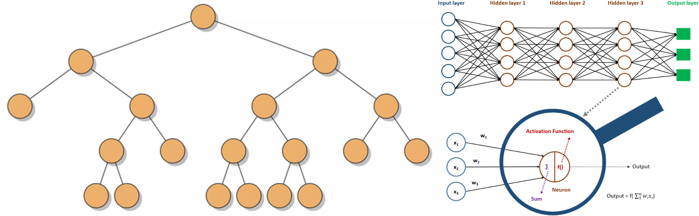 Nonlinear models
The type of the model plays an important role when generating features, so we will pay some attention to that.
Feature types
The following data types are most common:
- numeric
- categorical
- ordered categorical
- datetime
- bulk (images, sounds)
- complex (coordinates)
Some of these are called quantitative if they describe quantities, else qualitative if they describe some quality. Categorical data are usually qualitative (man or woman).
We will analyse in here numeric, categorical and datetime features and actions we can do on them to prepare these features for our machine learning models.
Numeric features
Here we will analyse some preprocessing steps we may use to prepare our data for the model.
Preprocessing: scaling
If we multiply a numeric feature with some constant, this is called scaling.
If we scale a single feature by multiplying it with a single constant we alter the relative proportion it has to other features, so this is not common.
It is very common to scale or normalize a feature as in the next examples:
Example: Scale to [0,1]
All the values at the end will be inside the range [0,1].
import pandas as pd
df = pd.DataFrame({'numbers': [ 1,2,3, 99]})
normalized_df=(df-df.min())/(df.max()-df.min())
normalized_df
Out:
  numbers
0   0.000000
1   0.010204
2   0.020408
3   1.000000
This operation is also called min-max scaling.
Example: standard normal distribution $\mathcal N(0,1)$
import pandas as pd
df = pd.DataFrame({'numbers': [ 1,2,3, 99]})
normalized_df=(df-df.mean())/df.std()
normalized_df
Out:
  numbers
0   -0.520545
1   -0.499929
2   -0.479314
3   1.499787
This operation is also called standard scaling.
Standard scaling and min-max scaling scale absolute distances. In case of outliers relative distances between outliers and other values will be huge.
How to process outliers then?
Preprocessing: outliers
In the previous case we had a numbers series 1,2,3,99:
import pandas as pd
df = pd.DataFrame({'numbers': [ 1,2,3, 99]})
Our assumption here was that 99 is an outlier. We can define outliers as those values outside of [Q1-1.5⋅IQR,Q3+1.5⋅IQR]. Here IQR is the Q3-Q1.
Clipping outliers is also called winsorization or anomaly removal.
To protect models from outliers, we can clip outlier values between two chosen values, usually the max and min values for a feature.
Another technique is to set them to NaN. In some cases we may ignore the records holding outliers.
Preprocessing: rank transform
Another way to deal with outliers is to rank our data:
from scipy.stats import rankdata
rankdata([0, 2, 3, 2]) # [1.  2.5 4.  2.5]
rankdata([0, 2, 3, 2], method='min') # [1 2 4 2]
rankdata([0, 2, 3, 2], method='max') # [1 3 4 3]
rankdata([0, 2, 3, 2], method='dense') # [1 2 3 2]
rankdata([0, 2, 3, 2], method='ordinal') # [1 2 4 3]
numpy doesn’t have such a convenient method like
rankdatafromscipy.
Preprocessing: math transforms
Another way to deal with outliers is to use special math transforms. We can use different math functions to transform the data:
- sigmoid function
- logit function
- log function
- power to $a$, where $a \in [0,1]$
This is especially valuable for neural networks.
Examples: Sigmoid and logit
# these are vectorized versions
from scipy.special import expit, logit
x = expit([-np.inf, -1.5, 0, 1.5, np.inf])
print(x) #[0.         0.18242552 0.5        0.81757448 1.        ]
x = logit(x) # [-inf -1.5  0.   1.5  inf]
print(x)
Example: All values between 0 and 1 except outliers much greater than 1
The next transforms will make the relative differences smaller:
l = [0.1, 0.9, 9]
np.sqrt(l)
Out:
array([0.31622777, 0.9486833 , 3.])
Another function we may use is log:
l = [0.1, 0.9, 9]
np.log(l)
Out:
array([-2.30258509, -0.10536052, 2.19722458])
Categorical features
First let’s make a short intro to distinguish categorical and ordered categorical features.
When categorical features do have a meaningful order as in the case of grades: A, B, C, D we can set the relations A > B, A > C, …, B > C and so on; these are ordered categorical features.
In case of simple categorical features such as sex values cannot be compared: man $\not \gt$ woman. This would be the regular categorical feature.
The order is the extra information.
Decision trees can utilize categorical features in an excellent way because they can split decisions based on different categorical values. Decision trees are great with ordered categorical features.
Non-tree models usually don’t benefit much from categorical features, unless they are ordered. This is why we create dummies then.
Categorical features encoding
The following examples are categorical feature encoding:
Example: Alphabetical label encoding
from sklearn.preprocessing import LabelEncoder
le = LabelEncoder()
le.fit(["paris", "paris", "tokyo", "amsterdam"])
print(list(le.classes_))
print(list(le.transform(["tokyo", "tokyo", "paris"])))
print(list(le.inverse_transform([2, 2, 1])))
Out:
['amsterdam', 'paris', 'tokyo']
[2, 2, 1]
['tokyo', 'tokyo', 'paris']
Example: Label encoding by appearance
import pandas as pd
lst = ["paris", "paris", "tokyo", "amsterdam"]
labels = pd.factorize(lst)
print(labels[0])
print(labels[1])
Out:
[0 0 1 2]
['paris' 'tokyo' 'amsterdam']
Example: Frequency encoding
import seaborn as sns
from scipy.stats import rankdata
ds = sns.load_dataset('iris')
freq_encoding = ds.species.value_counts(normalize=True)
freq_encoding
ds['FREQ_ENC'] = ds.species.map(freq_encoding)
ds['FREQ_ENC'].head()
Out:
0    0.333333
1    0.333333
2    0.333333
3    0.333333
4    0.333333
Example: One hot encoding
We use pandas.get_dummies but there is also a scikit-learn variant for the same called OneHotEncoder.
Try to use the get_dummies method because it is very simple to use.
import seaborn as sns
ds = sns.load_dataset('iris')
dummies = pd.get_dummies(pd.Series(ds.species))
ds = ds.join(dummies)
ds
Out:
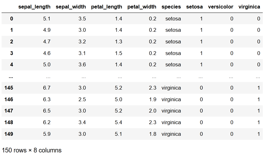
It is possible to make one hot encoding if you concatenate 2 string features and one hot encode that.
Example: Convert strings to category types
To create the model we need numerical inputs not strings, so we promote the following columns (that hold strings) to categories:
cat = ["MARTIAL_STATUS", "EDUCATION", "EMPLOYMENT", "GENDER" ]
for c in df.columns:
    if (df[c].dtype=='object'):
        df[c+"_cat"] = df[c].astype('category')
        df[c+"_cat"] = df[c+"_cat"].cat.codes
When working with Decision Trees and categorical features, label encoding is better than one hot encoding, because there is a meaning of category order.
This is especially true when the number of categorical features is big. If we have categorical features that are not ordered, we may order them the best we can.
Datetime features
Frequently we create sub features from dates like:
- day in week
- day in year
- month
- hour
- minutes
- seconds
- season
- holiday or no
- etc.
This would be nice to understand the repetitive patterns in the data.
Another approach would be to measure the time before some event, or after some event. For instance, the New Year event. This would be common for all the rows in the dataset.
Another approach is to track the time difference between two dates for each row. For instance, the day of the last transaction and the day of the last bank call. The difference between these two dates may be a good new feature.
Example: Check if a date is bad
pd.to_datetime('9999-10-01', format='%Y-%m-%d', errors='coerce')
Out:
NaT
It returns Not a Time (NaT). Here we are also converting strings to dates using to_datetime. Pandas can detect if a date is wrong.
Example: Check how many bad dates in a column
pd.isnull(pd.to_datetime(ds['CURRENT_JOB_DATE'], format='%Y-%m-%d', errors='coerce')).sum()
Out:
53
Handling missing values
What are missing values? The answer depends on how you understand what missing values are. Usually these are:
- blanks
- spaces
- strange big numbers such as -999
- default values such as 0
NaNorNaTvalues- undefined
To understand if a value is missing, you can check the histogram for data features. If it looks like the data is inside [0,1] range all the time and there are few exceptions with the value -1, these may be treated as missing values.
Maybe someone before set all the missing values to -1 already.
You can try with simple solution to replace the missing values with mean or median of the data, for that feature.