Bias Variance Noise trade off
- The machine learning models
- The dataset model
- The dataset model again
- The expected label (target)
- Hypothesis $h_D$
- Expected test error (given $h_D$)
- Expected hypothesis (given $\mathcal A$):
- Expected test error (given $\mathcal A$)
- Decomposition of the expected test error
- Final Formula
- Model complexity trade off
- Intuition on bias and variance
One of the most important formulas in statistics and machine learning is bias variance trade off. It actually generalizes to Bias, Variance Noise trade off here I will show how.
Engineering job is to find the equilibrium of these three, since intuitively if you make one of them smaller, the other two usually get bigger.
The following analysis will track one regression problem and explain the decomposition of the expected test error from the probabilistic approach.
The machine learning models
According to No Free Lunch Theorem every successful machine learning algorithm must make assumptions about the model.
In other words there is no single machine learning algorithm that works for all machine learning problems.
We write particular algorithm $h$ is a hypothesis drawn from a hypothesis class $\mathcal H$.
The dataset model
Let’s have a multivariate random variable or random vector $X$ and a target random variable $Y$.
The joint distribution of $X$ and $Y$ is also a random variable $D \sim P(X,Y)$.
We draw concrete dataset $\mathcal D$ from sample space with $n$ rows from $P(X,Y)^n$
The domain of random variable is called a sample space. This is a set of all possible outcomes, let’s define that.
The dataset model again
Let’s have the same dataset:
where:
- $y \in \mathbb{R}$ is our target or label
- $\boldsymbol{x} \in \mathbb{R}^d$ is our features vector ( $d$ columns)
- training dataset has $n$ inputs (rows)
$\mathbb R^d$ is the $d$-dimensional feature space, generally it may not be $\mathbb R$, but in here this is our simplified assumption.
We tackle a typical regression problem with MSE but the idea can generalize.
Specific quirk is assuming there is just a single realization $\mathcal D$ of a random variable $D$. Even though I can draw infinitely meany datasets $\mathcal D$ from $D$. For simplicity I will just write $D$ from now on. I need $D$ to be at the same time random variable (to estimate the first moment) and to be concrete dataset I work on.
The expected label (target)
If we are selling cars, there may be two exact cars, with the same equipment, but the target price may differ.
That different targets $y$ for the same feature vector $\boldsymbol x$ is what brings data inartistic noise.
This is why we need the expected target value $\bar y(\boldsymbol x)$ where $\boldsymbol x$ is a vector of features.
$\bar{y}(\boldsymbol x)=\mathbb E_{y \mid \boldsymbol{x}}[Y]=\int_{y} y P(y \mid \boldsymbol{x}) \partial y$
Check the noise part of the total error later on.
Hypothesis $h_D$
Since we have training dataset $D$ we may start the learning process.
$h_{D} = \mathcal A(D)$
Now, $D$ is a random variable and $\mathcal A$ is the algorithm so $h_D$ is also a random variable.
The specific meaning of this random variable $h_D$ is that it represents all the hypothesis from all different algorithm classes.
For instance hyperparameter tuning would be all the hypothesis and different algorithm classes would be KNN and DNN.
Now, it would be great if we can say what is the best class $h_D$? This is why we will from now on use the MSE loss metric (most common for regression problems).
Expected test error (given $h_D$)
$\begin{aligned}\mathbb E_{(\boldsymbol{x}, y) \sim P}\left[\left(h_{D}(\boldsymbol{x})-y\right)^{2}\right]=\int_{x}\int_{y}\left(h_{D}(\boldsymbol{x})-y\right)^{2} \operatorname{P}(\boldsymbol{x}, y) \partial y \partial \boldsymbol{x}\end{aligned}$
Expected hypothesis (given $\mathcal A$):
Note since there are different possible hypothesis on a dataset, we need the best one according to our metric (minimal loss).
We can think of the expected hypothesis and expected test error as well.
$\bar{h}=\mathbb E_{D \sim P^{n}}\left[h_{D}\right]=\int_{D} h_{D} \operatorname{P}(D) \partial D$
Expected test error (given $\mathcal A$)
$\mathbb E_{(\boldsymbol{x}, y) \sim P}\left[\left(h_{D}(\boldsymbol{x})-y\right)^{2}\right]=\int_{D} \int_{\boldsymbol{x}} \int_{y}\left(h_{D}(\boldsymbol{x})-y\right)^{2} \mathrm{P}(\boldsymbol{x}, y) \mathrm{P}(D) \partial \boldsymbol{x} \partial y \partial D$
Decomposition of the expected test error
\(\begin{aligned} \mathbb E_{\boldsymbol{x}, y, D}\left[\left(h_{D}(\boldsymbol{x})-y\right)^{2}\right] &=\mathbb E_{\boldsymbol{x}, y, D}\left[\left[\left(h_{D}(\boldsymbol{x})-\bar{h}(\boldsymbol{x})\right)+(\bar{h}(\boldsymbol{x})-y)\right]^{2}\right] \\ &=\mathbb E_{\boldsymbol{x}, D}\left[\left(\bar{h}_{D}(\boldsymbol{x})-\bar{h}(\boldsymbol{x})\right)^{2}\right]+2 \mathbb E_{\boldsymbol{x}, y, D}\left[\left(h_{D}(\boldsymbol{x})-\bar{h}(\boldsymbol{x})\right)(\bar{h}(\boldsymbol{x})-y)\right]+\mathbb E_{\boldsymbol{x}, y}\left[(\bar{h}(\boldsymbol{x})-y)^{2}\right] \end{aligned}\) The middle term of the above equation is 0 as we show below \(\begin{aligned} \mathbb E_{\boldsymbol{x}, y, D}\left[\left(h_{D}(\boldsymbol{x})-\bar{h}(\boldsymbol{x})\right)(\bar{h}(\boldsymbol{x})-y)\right] &=\mathbb E_{\boldsymbol{x}, y}\left[\mathbb E_{D}\left[h_{D}(\boldsymbol{x})-\bar{h}(\boldsymbol{x})\right](\bar{h}(\boldsymbol{x})-y)\right] \\ &=\mathbb E_{\boldsymbol{x}, y}\left[\left(\mathbb E_{D}\left[h_{D}(\boldsymbol{x})\right]-\bar{h}(\boldsymbol{x})\right)(\bar{h}(\boldsymbol{x})-y)\right] \\ &=\mathbb E_{\boldsymbol{x}, y}[(\bar{h}(\boldsymbol{x})-\bar{h}(\boldsymbol{x}))(\bar{h}(\boldsymbol{x})-y)] \\ &=\mathbb E_{\boldsymbol{x}, y}[0] \\ &=0 \end{aligned}\)
Returning to the earlier expression, we’re left with the variance and another term:
\[\mathbb E_{\boldsymbol{x}, y, D}\left[\left(h_{D}(\boldsymbol{x})-y\right)^{2}\right]=\underbrace{\mathbb E_{\boldsymbol{x}, D}\left[\left(h_{D}(\boldsymbol{x})-\bar{h}(\boldsymbol{x})\right)^{2}\right]}_{\text {Variance }}+\mathbb E_{\boldsymbol{x}, y}\left[(\bar{h}(\boldsymbol{x})-y)^{2}\right]\]We can break down the second term in the above equation as follows:
\[\begin{aligned} \mathbb E_{\boldsymbol{x}, y}\left[(\bar{h}(\boldsymbol{x})-y)^{2}\right] &=\mathbb E_{\boldsymbol{x}, y}\left[(\bar{h}(\boldsymbol{x})-\bar{y}(\boldsymbol{x}))+(\bar{y}(\boldsymbol{x})-y)^{2}\right] \\ &=\underbrace{\mathbb E_{\boldsymbol{x}, y}\left[(\bar{y}(\boldsymbol{x})-y)^{2}\right]}_{\text {Noise }}+\underbrace{\mathbb E_{\boldsymbol{x}}\left[(\bar{h}(\boldsymbol{x})-\bar{y}(\boldsymbol{x}))^{2}\right]}_{\text {Bias }^{2}}+2 \mathbb E_{\boldsymbol{x}, y}[(\bar{h}(\boldsymbol{x})-\bar{y}(\boldsymbol{x}))(\bar{y}(\boldsymbol{x})-y)] \end{aligned}\]The third term in the equation above is $0,$ as we show below:
\[\begin{aligned} \mathbb E_{\boldsymbol{x}, y}[(\bar{h}(\boldsymbol{x})-\bar{y}(\boldsymbol{x}))(\bar{y}(\boldsymbol{x})-y)] &=\mathbb E_{\boldsymbol{x}}\left[\mathbb E_{y \mid \boldsymbol{x}}[\bar{y}(\boldsymbol{x})-y](\bar{h}(\boldsymbol{x})-\bar{y}(\boldsymbol{x}))\right] \\ &=\mathbb E_{\boldsymbol{x}}\left[\mathbb E_{y \mid \boldsymbol{x}}[\bar{y}(\boldsymbol{x})-y](\bar{h}(\boldsymbol{x})-\bar{y}(\boldsymbol{x}))\right] \\ &=\mathbb E_{\boldsymbol{x}}\left[\left(\bar{y}(\boldsymbol{x})-\mathbb E_{y \mid \boldsymbol{x}}[y]\right)(\bar{h}(\boldsymbol{x})-\bar{y}(\boldsymbol{x}))\right] \\ &=\mathbb E_{\boldsymbol{x}}[(\bar{y}(\boldsymbol{x})-\bar{y}(\boldsymbol{x}))(\bar{h}(\boldsymbol{x})-\bar{y}(\boldsymbol{x}))] \\ &=\mathbb E_{\boldsymbol{x}}[0] \\ &=0 \end{aligned}\]Final Formula
Total error can be decomposed to bias, variance and noise.
Variance
How much the model output changes if you train on a different dataset set $D$?
This variance is the expectation of the squared difference from the hypothesis function on dataset $D$ and average hypothesis.
If we are over-specialized on some set $D$ we are overfitting.
Typically if the dataset becomes larger the variance should become smaller.
If I remove the outliers, I change the data distribution, and this can certainly help the variance decrease. This means I can use complex models, because variance decreased, and if I use complex models the bias will decrease.
Bias
Bias exists because your hypothesis functions are biased to a particular kind of solution. In other words, bias is inherent to your model.
Noise
How can we reduce noise? Noise depends on the number of features (feature space) so with more features can can help reducing the data inartistic noise.
Also noise is not a function of $D$, more data will not help reducing the noise.
However, here is the trade off, if I add more features, and make noise smaller, I will make the variance larger. This would be the features trade off.
Model complexity trade off
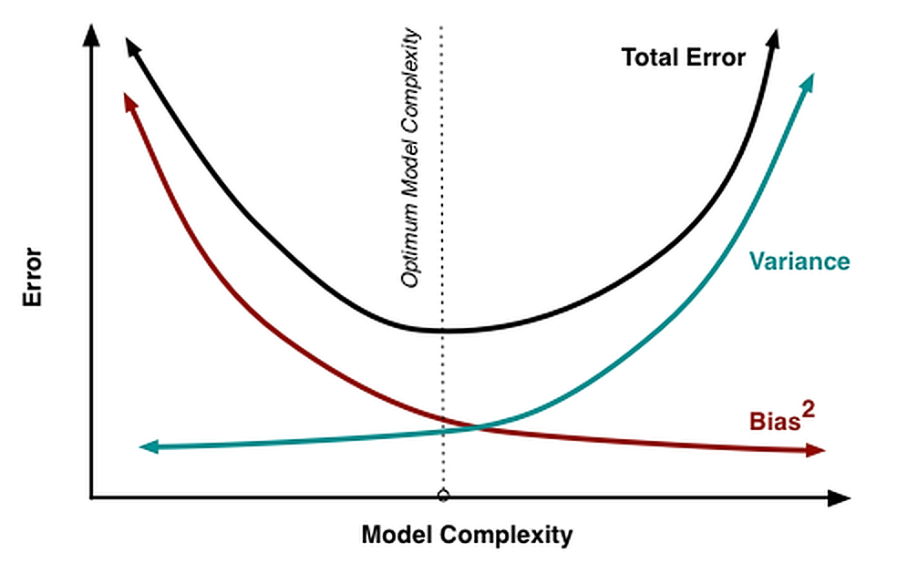
If we set the noise aside the bias variance tradeoff, is simple this.
We know as our model is more complex, it is capable to learn the train dataset specifics well, but it will overfit on a test dataset. The variance on a test dataset will be big. Simpler models cannot learn all the fine grains of the training dataset and because of that the variance will be lower.
It is completely opposite from the bias perspective. The model complexity, make the bias lower. This provides the intuition there is the optimal model complexity we are looking for.
Intuition on bias and variance
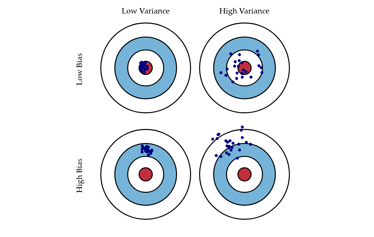
How to reduce high variance?
You can detect high variance if the training error is much lower than test error.
If this is the case:
- add more training data
- reduce model complexity
- use bagging
How to reduce the high bias?
If you are not in high variance mode your train and test errors should be close.
If you have high bias: the model being used is not robust enough to produce an accurate prediction.
If this is the case:
- use complex model
- add features
- use boosting