Bayesian prerequisites | Sampling
- Sampling
- Importance Sampling
- Rejection sampling
- MCMC
- Gibbs sampling
- Metropolis-Hastings
- Hamiltonian Monte Carlo
- NUTS
- MCMC software
- Compare Sampling and Variational Inference Algorithms
Sampling
Sampling algorithms produce answers by generating random numbers from a distribution of interest.
One fundamental problem in machine learning is to generate samples $x_i$ from some distribution $p(x)$.
\[\{x_i\}_{i=1}^n \sim p({x}) \tag{1}\]$p(x)$ is notation of continuous and $P(x)$ of discrete distribution.
We frequently search for the expectation $\large \mu$ of any function $f: \mathbb R \rightarrow \mathbb{R}$ under that distribution:
\[\mu \equiv \mathbb{E}_{p}[f(x)]=\int_{\mathbb R} f(x) p(x) d x \tag{2}\]Monte Carlo method is when we use the samples $x_i$ to find the expectation of $f$:
\[\hat{\mu} \equiv \frac{1}{n} \sum_{i=1}^{n} f\left(x_{i}\right) \tag{3}\]Monte Carlo sampling depends on the sample size $\large n$ and should not depend on the dimensionality of the random variable $X$ or cardinality.
Two very popular Monte Carlo methods are Importance and Rejection sampling. After that we cover a few Markov Chain Monte Carlo methods including Gibbs and Metropolis-Hastings sampling.
My idea is to provide a basic classification and intuition for the methods. You may check the reference materials for the strict mathematical definitions and more details.
Importance Sampling
We only know to sample from few distributions including Uniform and Gaussian. Distribution $p(x)$ may not be one of them. So how to sample from $p(x)$?
Importance sampling takes an easy-to-sample distribution $q(x)$ into play from where we generate samples.
We use un-normalized distribution $\tilde q(x)$ in general case to generate $n$ samples and then we compute:
\[w_{i}=\frac{\tilde{p}\left(x_i\right)}{\tilde{q}\left(x_i\right)}\]In there $\tilde p(x)$ is also an un-normalized distribution.
The expectation of $f$ is then:
\[\hat{\mu} \equiv \frac{ \begin{aligned} \sum_{i=1}^{n} w_{i} f\left(x_{i}\right)\end{aligned}}{\begin{aligned} \sum_{i=1}^{n} w_{i}\end{aligned}}\]As we say importance sampling is not a method to direct sample from distribution $p$, instead we used another easy-to-sample distribution $q$.
Importance sampling methods are originally designed for integral approximations such as approximating intractable posterior distributions or marginal likelihoods.
Sampling methods from a distribution with density $p$ are used in these most common cases:
- to get an idea about this distribution
- to solve an integration problem related to it
- to solve optimization problem related to it
Rejection sampling
Accept-reject or rejection sampling method is used to sample from hard-to-sample distributions. In here we sample based on acceptance or rejection.
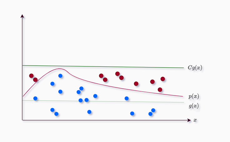
Assuming $p(x)$ is a hard-to-sample distribution and $g(x)$ is uniform distribution. We find the constant $C$ such that:
\[Cg(x) > p(x)\]Anything above the $p(x)$ will be rejected (red) and anything below will be accepted (blue), thus the name.
The only condition we are using is one If condition to check if the current sample is greater than $p(x)$, or smaller or equal to $p(x)$.
We frequently consider the case where $q$ is uniform, but it is possible to use any easy-to-sample distribution. $q$ is known as proposal distribution.
Rejection sampling doesn’t work well in dimensions.
MCMC
Markov chain Monte Carlo methods are extensions of previous methods when previous methods are slow to compute.
This is why when we think of sampling methods we often think of MCMC.
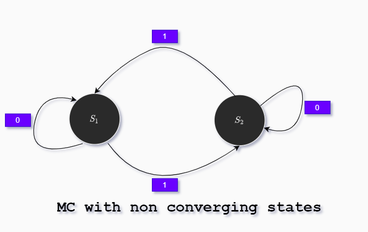
Markov chain is a mathematical system (also called random process) very similar to finite state machines where we define state transitions with assigned probabilities and we write e.g. $S_1 \rightarrow S_2$ (state $S_1$ transition to state $S_2$).
The defining characteristic of a Markov chain is that no matter how the process arrived at its present state, the probability of possible future states are fixed.
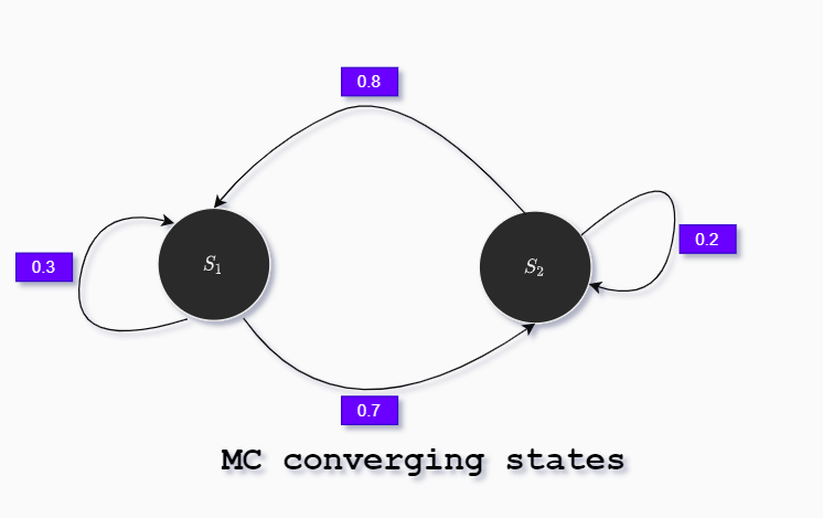
We may use the matrix notation to describe the random process of Markov chain:
\[P=\left[\begin{array}{ll} 0.3 & 0.7 \\ 0.8 & 0.2 \end{array}\right]\]At each time interval there is a fixed probability to switch to any state. After many time steps states we may or may not converge to stationary distribution.
The next Markov chain will not converge to a stationary probability distribution (states are altered each timestep):
Opposite the next Markov chain will converge to stationary distribution:
To calculate the stationary states we use the following Python code:
def switch_state(current):
    '''
    returns the new state
    '''
    if current == 1:
        if np.random.uniform() > 0.3:
            return 2
        else:
            return 1

    if current == 2:
        if np.random.uniform() > 0.2:
            return 1
        else:
            return 2

current = 1
lst = [1]
M=100000
'''
100.000 different timesteps
'''
for i in range(M):
    current = switch_state(current)
    lst.append(current)

print(lst.count(1))
Out:
53368
This means: about 53% we are in $S_1$ and 47% in state $S_2$.
Another way to work on the same problem is this matrix calculus:
import numpy as np
from numpy import linalg as LA

def simulate_MC(x_0, P, k):
    for i in range(k):
        P_k = LA.matrix_power(P, i)
        x_k = np.dot(x_0, P_k)
        print(f'x^({i}) = {x_k[0]} {x_k[1]}')

P = np.array([[0.3, 0.7], [0.8, 0.2]])
state = np.array([1, 0]) # init

simulate_MC(state, P, 20)
Out:
x^(0) = 1.0 0.0
x^(1) = 0.3 0.7
x^(2) = 0.6499999999999999 0.35
x^(3) = 0.475 0.5249999999999999
x^(4) = 0.5624999999999999 0.43749999999999994
x^(5) = 0.5187499999999998 0.48124999999999996
x^(6) = 0.5406249999999998 0.4593749999999999
x^(7) = 0.5296874999999999 0.47031249999999997
x^(8) = 0.5351562499999998 0.4648437499999999
x^(9) = 0.5324218749999998 0.4675781249999999
x^(10) = 0.5337890624999998 0.46621093749999987
x^(11) = 0.5331054687499999 0.4668945312499999
x^(12) = 0.5334472656249998 0.46655273437499983
x^(13) = 0.5332763671874997 0.46672363281249984
x^(14) = 0.5333618164062497 0.4666381835937498
x^(15) = 0.5333190917968748 0.4666809082031248
x^(16) = 0.5333404541015622 0.4666595458984373
x^(17) = 0.5333297729492185 0.4666702270507811
x^(18) = 0.5333351135253903 0.46666488647460913
x^(19) = 0.5333324432373043 0.4666675567626951
As you may note we have the exact same result as in the first Python example.
You may think this has to have something with the init state, but if you alter the init state: state = np.array([0.5, 0.5]) # init we get the same result.
We found what is called the stationary distribution of states and frequently we denote it with $\pi$. The first Python example is simple Monte Carlo and the second is Markov chain Monte Carlo method. The first example had 100000 iterations while the second method had just 20 iterations. In general MCMC perform faster than naive Monte Carlo.
The math behind MCMC:
\[\begin{aligned} \pi P &= \pi \\ \pi(P-I) &= 0 \end{aligned}\]This would be formal expression of sampling:
\[\begin{aligned} \mathbb{E}_{p(x)} f(x) & \approx \frac{1}{M} \sum_{s=1}^{M} f(x_{s}) \\ x_{s} & \sim p(x) \end{aligned}\]If here:
- $p(x)$ is the distribution we sample from
- We build Markov chains that converge to $p(x)$.
- we start from any state
- we simulate for many (say $M$ = 10.000) time steps
Nice thing with MCMC:
- easy to implement
- easy to parallelize
- unbiased (the higher M better convergence)
- great for expected values
Possible problem:
- sometimes not sufficiently accurate (we need great number of samples $M$ to reach some accuracy)
Examples where we use MCMC:
- Full Bayesian inference (numerical integration over latent variables)
- M-step of EM algorithm
- Sampling from a probability distribution (e.g. expected values)
Now we will explain a few MCMC sampling types.
Gibbs sampling
Gibbs sampling is sampling from a $N-$dimensional distribution where single iteration means sampling $N\times$ in 1d.
After some number of iterations we get a sample that converges to the original distribution.
Example: 3 dimensional case.
If $X_{state}^{time- step}$ is our notation, and our initial state is $(x^0_1, x^0_2, x^0_3)$.
In time-step 1:
\[\begin{aligned} x_{1}^{1} & \sim p\left(x_{1} \mid x_{2}=x_{2}^{0}, x_{3}=x_{3}^{0}\right) \\ x_{2}^{1} & \sim p\left(x_{2} \mid x_{1}=x_{1}^{1}, x_{3}=x_{3}^{0}\right) \\ x_{3}^{1} & \sim p\left(x_{3} \mid x_{1}=x_{1}^{1}, x_{2}=x_{2}^{1}\right) \end{aligned}\]In time-step $k+1$:
\[\begin{aligned} x_{1}^{k+1} & \sim p\left(x_{1} \mid x_{2}=x_{2}^{k}, x_{3}=x_{3}^{k}\right) \\ x_{2}^{k+1} & \sim p\left(x_{2} \mid x_{1}=x_{1}^{k+1}, x_{3}=x_{3}^{k}\right) \\ x_{3}^{k+1} & \sim p\left(x_{3} \mid x_{1}=x_{1}^{k+1}, x_{2}=x_{2}^{k+1}\right) \end{aligned}\]As you may see for our 3D case we have 3 steps (states) per time state. Gibbs sampling is easy to implement, but it is relatively slow when dimensionality is big.
We cannot parallelize Gibbs sampling per time step.
Metropolis-Hastings
Metropolis-Hastings algorithm is MCMC method for obtaining a sequence of random samples from a probability distribution $p(x)$ from which direct sampling is difficult.
MH algorithm works by simulating a Markov chain, whose stationary distribution is $p(x)$ so in the long run, the samples from the Markov chain should look like the samples from distribution $p(x)$.
This idea is sometimes called rejection sampling applied to Markov chains.
Metropolis-Hastings is a six step algorithm:
- start with a random sample
- determine the probability density associated with the sample
- propose a new, arbitrary sample (and determine its probability density)
- compare densities (via division), quantifying the desire to move
- generate a random number, compare with desire to move, and decide: move or stay
- repeat
Requirement: For a given probability density function $p(x)$, we only require that we have a function $f(x)$ that is proportional to $p(x)$!
MH is extremely useful when sampling posterior distributions in Bayesian inference where the marginal likelihood (the denominator) is hard to compute.
Hamiltonian Monte Carlo
Hamiltonian Monte Carlo (HMC) is special case of Metropolis-Hastings algorithm that uses proposals.
Computing proposals is complicated and demanding, but often compensated by achieving high approximation accuracy.
Hamiltonian Monte Carlo avoids the random walk behavior and sensitivity to correlated parameters by taking a series of steps informed by first-order gradient information.
These features allow HMC to converge in high-dimension distributions better than Metropolis-Hastings or Gibbs sampling.
Gibbs sampling is considered as a special case of Metropolis-Hastings.
HMC performance is highly sensitive to:
- step size $\epsilon$
- desired number of steps $L$.
In particular, if $L$ is too small then the algorithm exhibits undesirable random walk behavior, while if $L$ is too large the algorithm wastes computation.
NUTS
No-U-Turn Sampler (NUTS), an extension to HMC that eliminates the need to set a number of steps $L$. NUTS uses a recursive algorithm to build a set of likely candidate points that spans a wide swath of the target distribution, stopping automatically when it starts to double back and retrace its steps.
Empirically, NUTS perform at least as efficiently as and sometimes more efficiently than a well tuned standard HMC method, without requiring user intervention or costly tuning runs.
MCMC software
Here is a short overview of MCMC software:
- BUGS
- JAGS
- PyMC
- Stan
The first-made software for MCMC was BUGS: Bayesian inference using Gibbs sampling, made in the 1990s.
BUGS uses BUGS language to specify the model and uses Gibbs sampling method.
Inspired by BUGS, a parallel effort called JAGS or Just another Gibbs sampler had integration with R language.
PyMC uses Metropolis-Hastings sampler. It is now present as a Python package for defining stochastic models and constructing Bayesian posterior samples. PyMC is possibly more famous for modeling Gaussian processes.
There is also the language called Stan. Stan allows flexible model specification (more flexible than BUGS). Stan includes the option for MCMC using HMC and NUTS. The Stan software integrates with R, Python, MATLAB, Julia, and Stata.
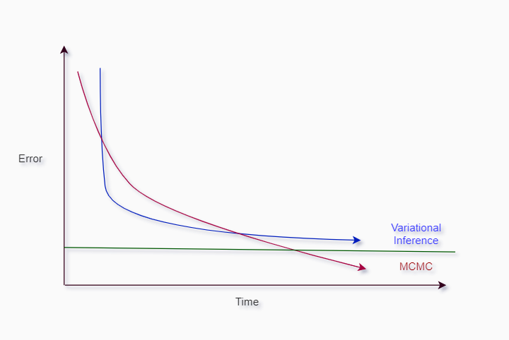
Compare Sampling and Variational Inference Algorithms
Variational algorithms are a family of techniques for approximating intractable integrals arising in Bayesian inference and machine learning. They treat inference problems as optimization.
Although sampling algorithms were invented first ( during the II world war ), variational inference methods dominates the field because these methods are fast.
VI methods are invented in sixties and these are approximation algorithms.
Short feedback of the two techniques:
- VI runs faster in most cases
- VI often cannot find globally optimal solution, can converge to a solution up to a certain boundary
- Sampling methods are more precise and can find globally optimal solution
- Both methods can run in parallel (on multiple CPUs/GPUs).
Reference: