Bayesian prerequisites | Gaussian
In Bayesian statistics Gaussian or normal distribution is frequent. Gaussian distribution has closed-form solution for marginal and conditional dependencies which is neat.
Parameters
In classical probability all the distributions are implicitly conditioned on $\theta$, where $\theta$ are some parameters. These parameters are treated as unknown constants.
Classical notation that $X$ depends on $\theta$ where $\theta$ is a parameter would be: $P(X ; \theta) = P_{\theta}(X)$.
In Bayesian probability, you may be surprised, unknown constants don’t exist, these are promoted to random variables.
$P(X \mid \theta)$ where both $X$ and $\theta$ are random variables means $\theta$ is unknown random variable, and we cannot just write $P(X)$ because $X$ is not independent random variable.
Given the importance of the Gaussian distributions, here we consider likelihood methods for fitting a Gaussian to data.
Gaussian distribution is important even for defining priors. Goodfellow et al. suggests that priors should come from high-entropy distributions, such as the normal distribution, because this reflects uncertainty in the parameters.
Univariate Gaussian PDF
For a univariate random variable, the Gaussian distribution has a density that is given by: \(p\left(x \mid \mu, \sigma^{2}\right)=\frac{1}{\sqrt{2 \pi \sigma^{2}}} \exp \left(-\frac{(x-\mu)^{2}}{2 \sigma^{2}}\right)\)
Univariate Gaussian distribution is fully specified by its mean and covariance.
Multivariate Gaussian PDF
Multivariate distributions are difficult to deal with computationally, except in special case like for multivariate Gaussian, for which marginals and normalization constants can be computed.
The multivariate Gaussian distribution of dimension $d$ where $\boldsymbol{x} \in \mathbb R^d$ is fully characterized by a mean vector $\boldsymbol{\mu} \in \mathbb R^d$ and a covariance matrix $\boldsymbol{\Sigma} \in \mathbb{R}^{d \times d}$ and is defined as: \(p(\boldsymbol{x} \mid \boldsymbol{\mu}, \boldsymbol{\Sigma})=(2 \pi)^{-\frac{d}{2}}|\boldsymbol{\Sigma}|^{-\frac{1}{2}} \exp \left(-\frac{1}{2}(\boldsymbol{x}-\boldsymbol{\mu})^{\top} \boldsymbol{\Sigma}^{-1}(\boldsymbol{x}-\boldsymbol{\mu})\right)\)
We write $p(\boldsymbol{x})=\mathcal{N}(\boldsymbol{x} \mid \boldsymbol{\mu}, \boldsymbol{\Sigma})$ or $X \sim \mathcal{N}(\boldsymbol{\mu}, \boldsymbol{\Sigma})$.
Special case called standard normal distribution is when $\boldsymbol{\mu}=0$ and $\boldsymbol{\Sigma}=I$.
Every real symmetric matrix such as covariance matrix $\boldsymbol{\Sigma} \in \mathbb{R}^{d \times d}$ has an eigendecomposition:
$\boldsymbol{\Sigma}=R\Lambda R^{\top}$, where $R$ and $R^{\top}$ are orthonormal matrices and $R^{\top}=R^{-1}$ or $R^{\top}R = I$.
Covariance matrix intuition
We will now show what is the meaning of this covariance matrix decomposition.
If we have data matrix $X \in \mathbb{R}^{n \times d}$ we can compute covariance matrix of the data with $n$ degrees of freedom.
\[\boldsymbol{\Sigma}=\frac{1}{n} \sum_{i=1}^{n}\left(X_{i}-\bar{X}\right)\left(X_{i}-\bar{X}\right)^{\top}\]For $X \in \mathbb{R}^{d \times n}$ we would have:
\[\boldsymbol{\Sigma}=\frac{1}{n} \sum_{i=1}^{n}\left(X_{i}-\bar{X}\right)^{\top}\left(X_{i}-\bar{X}\right)\]For the data with zero mean we can rewrite this even more compact: \(\boldsymbol{\Sigma}=\frac{X X^{\top}}{N}\)
Here is the covariance matrix of two random variables $X$ and $Y$:
\[\boldsymbol{\Sigma}=\left(\begin{array}{ll} \sigma(x, x) & \sigma(x, y) \\ \sigma(y, x) & \sigma(y, y) \end{array}\right)\]when the $X$ and $Y$ are uncorrelated we have 2D Gaussian noise.
\[\boldsymbol{\Sigma}=\left(\begin{array}{cc}\sigma_{x}^{2} & 0 \\ 0 & \sigma_{y}^{2}\end{array}\right)\]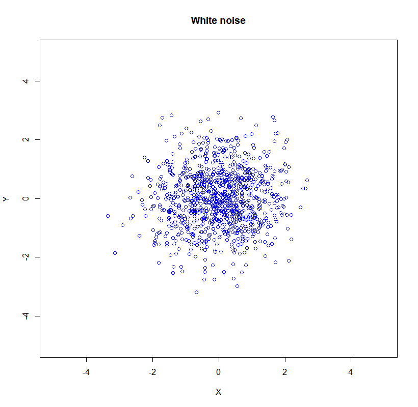
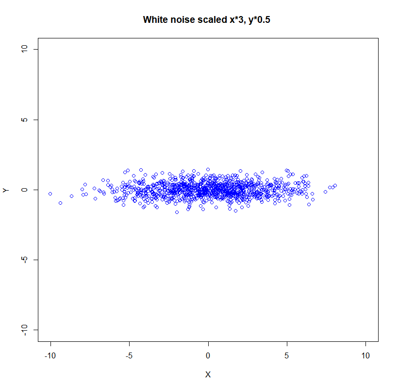
If we scale the data:
\[\boldsymbol{\Sigma}=\left(\begin{array}{cc}\left(s_{x} \sigma_{x}\right)^{2} & 0 \\ 0 & \left(s_{y} \sigma_{y}\right)^{2}\end{array}\right)\]the new picture is:
Now let’s rotate the data for the $\theta$ angle:
\[R=\left(\begin{array}{cc}\cos (\theta) & -\sin (\theta) \\ \sin (\theta) & \cos (\theta)\end{array}\right)\]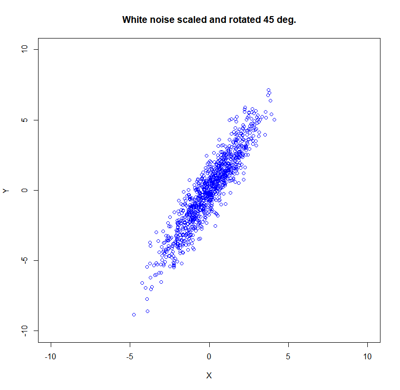
Here is the showcase in R
set.seed(1000)
X<- rnorm(1000, mean=0, sd=1)
Y<- rnorm(1000, mean=0, sd=1)
plot(X,Y, xlim=c(-5,5),ylim=c(-5,5), col='blue', lwd = 1,
     main = 'White noise', xlab = 'X', ylab = 'Y')

X <- X - mean(X)
Y <- Y - mean(Y)
X <- X*3
Y <- Y*0.5

plot(X,Y, xlim=c(-10,10),ylim=c(-10,10), col='blue', lwd = 1,
     main = 'White noise scaled', xlab = 'X', ylab = 'Y')


theta = (60*2*pi/360)

Xr <- X*cos(theta) - Y*sin(theta)
Yr <- X*sin(theta) + Y*cos(theta)
plot(Xr,Yr, xlim=c(-10,10),ylim=c(-10,10), col='blue', lwd = 1,
     main = 'White noise scaled and rotated 45 deg.', xlab = 'X', ylab = 'Y')
The covariance matrix is property of the data. We can factorize the covariance matrix into rotation and scaling.
$\boldsymbol{\Sigma}=R S S R^{-1} =R\Lambda R^{\top}$ and we had that before. This shows we can explicitly decompose covariance matrix into rotation and scaling. Here $\Lambda = diag(\lambda_1,…,\lambda_d)$ in the case of covariance matrix all eigenvalues $\lambda$ are positive, assuming $X$ is full rank matrix.
Further, we can calculate covariance matrix of any linear transformation.
We can also generalize if we would reason in terms:
\[\boldsymbol{y} = \Lambda^{-\frac{1}{2}}R^{\top}(\boldsymbol x-\boldsymbol{\mu})\]and show a multivariate Gaussian as a shifted, scaled and rotated version of a standard (zero mean, unit covariance) Gaussian.
\[(\boldsymbol{x}-\boldsymbol{\mu})^{\top} \boldsymbol{\Sigma}^{-1}(\boldsymbol{x}-\boldsymbol{\mu})=(\boldsymbol{x}-\boldsymbol{\mu})^{\top} \boldsymbol{E} \boldsymbol{\Lambda}^{-1} \boldsymbol{E}^{\boldsymbol{\top}}(\boldsymbol{x}-\boldsymbol{\mu})=\boldsymbol{y}^{\top} \boldsymbol{y}\]n.b.:
- center is given by the mean
- the rotation by the eigenvectors
- and the scaling by the square root of the eigenvalues
In the R example we started form the Gaussian Standard Normal data, but we can easily use the next trick to normalize our data:
X <- (X - mean(X))/sd(X)
The last trick is backpropagation algorithm best friend.
Sum of independent Gaussians
For the two independent vector random variables $X, Y \sim \mathcal{N}(\boldsymbol{\mu} \mid \boldsymbol{\Sigma})$ joint distribution $p(\boldsymbol x,\boldsymbol y) =p(\boldsymbol x)p(\boldsymbol y)$.
Then: \(p(\boldsymbol{x}+\boldsymbol{y})=\mathcal{N}\left(\boldsymbol{\mu}_{\boldsymbol{x}}+\boldsymbol{\mu}_{\boldsymbol{y}}, \boldsymbol{\Sigma}_{x}+\boldsymbol{\Sigma}_{\boldsymbol{y}}\right)\)
Or more general: \(p(a \boldsymbol{x}+b \boldsymbol{y})=\mathcal{N}\left(a \boldsymbol{\mu}_{x}+b \boldsymbol{\mu}_{y}, a^{2} \boldsymbol{\Sigma}_{x}+b^{2} \boldsymbol{\Sigma}_{y}\right)\)
Product of two Gaussians
The product of two Gaussians: \(\mathcal{N}\left(\boldsymbol{x} \mid \boldsymbol{\mu}_{1}, \boldsymbol{\Sigma}_{1}\right) \mathcal{N}\left(\boldsymbol{x} \mid \boldsymbol{\mu}_{2}, \boldsymbol{\Sigma}_{2}\right)=\mathcal{N}(\boldsymbol{x} \mid \boldsymbol{\mu}, \boldsymbol{\Sigma}) \frac{\exp \left(-\frac{1}{2}\left(\boldsymbol{\mu}_{1}-\boldsymbol{\mu}_{2}\right)^{\top} \boldsymbol{S}^{-1}\left(\boldsymbol{\mu}_{1}-\boldsymbol{\mu}_{2}\right)\right)}{\sqrt{\operatorname{det}(2 \pi \boldsymbol{S})}}\)
So mean and covariance are given by: \(\boldsymbol{\mu}=\boldsymbol{\Sigma}_{1} \mathbf{S}^{-1} \boldsymbol{\mu}_{2}+\boldsymbol{\Sigma}_{2} \mathbf{S}^{-1} \boldsymbol{\mu}_{1} \quad \boldsymbol{\Sigma}=\boldsymbol{\Sigma}_{1} \mathbf{S}^{-1} \boldsymbol{\Sigma}_{2}\)
where \(\mathbf{S} \equiv \boldsymbol{\Sigma}_{1}+\boldsymbol{\Sigma}_{2}\)
Gaussian mixture mean and variance
Let’s check two univariate Gaussian densities: \(p(x)=\alpha p_{1}(x)+(1-\alpha) p_{2}(x)\)
The mean of the mixture density $p(x)$ is given by the weighted sum of the means of each random variable: \(\mathbb{E}[x]=\alpha \mu_{1}+(1-\alpha) \mu_{2}\)
The variance of the mixture density $p(x)$ is given by: \(\mathbb{V}[x]=\left[\alpha \sigma_{1}^{2}+(1-\alpha) \sigma_{2}^{2}\right]+\left(\left[\alpha \mu_{1}^{2}+(1-\alpha) \mu_{2}^{2}\right]-\left[\alpha \mu_{1}+(1-\alpha) \mu_{2}\right]^{2}\right)\)
Linear transform of Gaussian
If we have linear transform: $\boldsymbol{y}=\boldsymbol{T x}+\gamma$
where \(\boldsymbol{x} \perp \gamma, \gamma \sim \mathcal{N}(\boldsymbol{\mu}, \boldsymbol{\Sigma}), \boldsymbol{x} \sim \mathcal{N}(\boldsymbol{\mu}_{x},\boldsymbol{\Sigma}_{x})\)
The marginal $p(\boldsymbol{y})=\int_{\boldsymbol{x}} p(\boldsymbol{y} \mid \boldsymbol{x}) p(\boldsymbol{x})$ is a Gaussian \(p(\boldsymbol{y})=\mathcal{N}\left(\boldsymbol{y} \mid \boldsymbol{T} \boldsymbol{\mu}_{x}+\boldsymbol{\mu}, \boldsymbol{T} \boldsymbol{\Sigma}_{x} \boldsymbol{T}^{\top}+\boldsymbol{\Sigma}\right)\)
Entropy of Gaussian
$p(\boldsymbol x) = \mathcal{N}(\boldsymbol x \mid \mu, \Sigma)$ is our PDF entropy is given by: \(H \equiv- \mathbb E_{p(\boldsymbol x)} \log p(\boldsymbol x) = \int_{\mathbb R^d} p(\boldsymbol x) \log p(\boldsymbol x) = \frac{1}{2} \log \operatorname{det}(2 \pi \Sigma)+\frac{d}{2}\)
Translated, scaled, rotated random variable
This is the case when $\boldsymbol{y}= \boldsymbol{Ax}$, we cam simple compute the new distribution:
\[\mathbb{E}[\boldsymbol{y}]=\mathbb{E}[\boldsymbol{A} \boldsymbol{x}]=\boldsymbol{A} \mathbb{E}[\boldsymbol{x}]=\boldsymbol{A} \boldsymbol{\mu}\] \[\mathbb{V}[\boldsymbol{y}]=\mathbb{V}[\boldsymbol{A} \boldsymbol{x}]=\boldsymbol{A} \mathbb{V}[\boldsymbol{x}] \boldsymbol{A}^{\top}=\boldsymbol{A} \boldsymbol{\Sigma} \boldsymbol{A}^{\top}\] \[p(\boldsymbol{y})=\mathcal{N}\left(\boldsymbol{y} \mid \boldsymbol{A} \boldsymbol{\mu}, \boldsymbol{A} \boldsymbol{\Sigma} \boldsymbol{A}^{\top}\right)\]Applications
Gaussian noise when MLE
If we model noise with Gaussian distribution for maximum likelihood estimation will have a closed-form analytic solution:
\[\begin{aligned} \mathcal{L}(\boldsymbol{\theta}) &=-\sum_{n=1}^{N} \log p\left(y_{n} \mid \boldsymbol{x}_{n}, \boldsymbol{\theta}\right)=-\sum_{n=1}^{N} \log \mathcal{N}\left(y_{n} \mid \boldsymbol{x}_{n}^{\top} \boldsymbol{\theta}, \sigma^{2}\right) \\ &=-\sum_{n=1}^{N} \log \frac{1}{\sqrt{2 \pi \sigma^{2}}} \exp \left(-\frac{\left(y_{n}-\boldsymbol{x}_{n}^{\top} \boldsymbol{\theta}\right)^{2}}{2 \sigma^{2}}\right) \\ &=-\sum_{n=1}^{N} \log \exp \left(-\frac{\left(y_{n}-\boldsymbol{x}_{n}^{\top} \boldsymbol{\theta}\right)^{2}}{2 \sigma^{2}}\right)-\sum_{n=1}^{N} \log \frac{1}{\sqrt{2 \pi \sigma^{2}}} \\ &=\frac{1}{2 \sigma^{2}} \sum_{n=1}^{N}\left(y_{n}-\boldsymbol{x}_{n}^{\top} \boldsymbol{\theta}\right)^{2}-\sum_{n=1}^{N} \log \frac{1}{\sqrt{2 \pi \sigma^{2}}} \end{aligned}\]Simple linear regression and Gaussian noise
In here we consider linear functions $f: \mathbb{R} \rightarrow \mathbb{R}$
\[y=x \theta+\epsilon, \quad \epsilon \sim \mathcal{N}\left(0, \sigma^{2}\right)\]The parameter $\theta$ is know as the slope.
Maximum likelihood estimator for the slope parameter is given:
\(\theta_{\mathrm{ML}}=\left(\boldsymbol{x}^{\top} \boldsymbol{x}\right)^{-1} \boldsymbol{x}^{\top} \boldsymbol{y}=\frac{\boldsymbol{x}^{\top} \boldsymbol{y}}{\boldsymbol{x}^{\top} \boldsymbol{x}}\) where $\boldsymbol{x}=\left[x_{1}, \ldots, x_{n}\right]^{\top} \in \mathbb{R}^{n}, \boldsymbol{y}=\left[y_{1}, \ldots, y_{n}\right]^{\top} \in \mathbb{R}^{n}$