Activation functions
- Identity
- Binary step
- ReLU
- ReLU6
- Leaky ReLU
- ELU
- CELU
- SELU
- GELU
- Sigmoid
- Hard Sigmoid
- Tanh
- SoftSign
- HardTanh
- Swish
- Softplus
- Mish
Activation functions are by default nonlinear functions.
Why do we need nonlinear activation functions?
If we would just have linear activation functions to stack neural network layers the final output will again be a linear function of the input.
Nonlinear means that the output cannot be reproduced from a linear combination of the inputs.
Without a nonlinear activation function neural network with any number of layers would behave like a single-layer perceptron.
The most important features to track for the specific activation functions are:
- function input range
- output range
- if function is monotonic
- number of kinks
- what is the derivative of a function
- if derivative is monotonic
I will shortly cover some of the functions present in PyTorch:
Identity
Very simple function:
$f(x) = x$
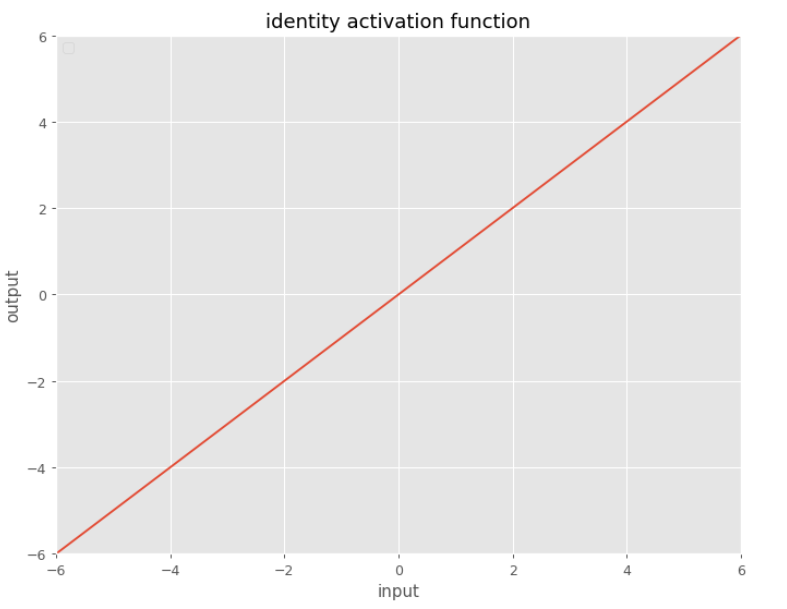
Has a very simple derivative. When we deal with activation functions, usually we like to have a nice derivative for the activation function.
The problem with this function, it will not introduce nonlinearity. To do that we can use hardtanh that works surprisingly well for many tasks.
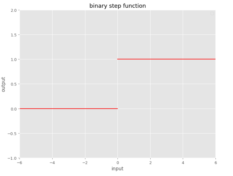
Binary step
Defined super simple this is one of the most basic functions:
The problem with this function is: derivate is not defined for $x=0$.
ReLU
$f\left(x\right) = \max\left(0, x\right)$
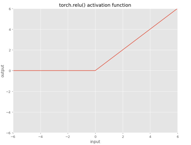
Rectified Linear Units, or ReLUs, are the most common activation functions. Linearity in the positive dimension has the attractive property that it prevents non-saturation of gradients (contrast with sigmoid activations), although for half of the real line its gradient is zero.
In PyTorch you just use torch.relu()
ReLU6
One specific variant of ReLU with two kinks is ReLU6:
$f(x)=min(max(0,x),6)$
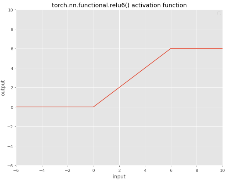
In here for inputs greater than 6 there will be no gradients.
Leaky ReLU
By default the slope is $0.01$ as in the formula, in the image the slope is $0.1$.
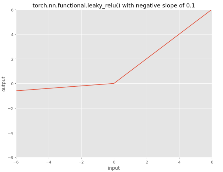
Leaky Rectified Linear Unit, or Leaky ReLU, is based on a ReLU, but it has a small slope for negative values instead of a flat slope.
The slope coefficient is determined before training, (not during training). This type of activation function is popular where we may suffer from sparse gradients, for example training GANs (Generative Adversarial Networks).
There is one modification of Leaky ReLU called parametrized Leaky ReLU:
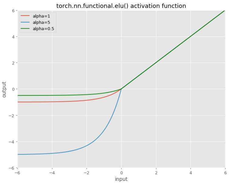
ELU
Or:
$\mathrm{ELU}(x)=\max (0, x)+\min (0, \alpha *(\exp (x)-1))$
ELU is another soft version of ReLU where you can control the parameter $\alpha$. If parameter $\alpha$ goes closer to zero we are getting even “closer” to ReLU. By default $\alpha=1$.
CELU
Very similar to ELU is CELU but now the exponent is also under the influence of the parameter $\alpha$.
$\operatorname{CELU}(x)=\max (0, x)+\min (0, \alpha *(\exp (x / \alpha)-1))$
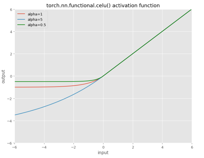
This function is continuously differentiable, thus the name.
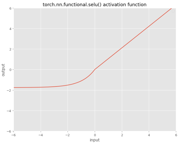
SELU
$\operatorname{SELU}(x)= \mathsf {scale} *(\max (0, x)+\min (0, \alpha *(\exp (x)-1)))$
with $\alpha=1.6732632423543772848170429916717$ and $\mathsf {scale}=1.0507009873554804934193349852946$
GELU
$\begin{aligned} & f(x) = \frac{1}{2} x\left(1+\operatorname{erf}\left(\frac{x}{\sqrt{2}}\right)\right) =& x \Phi(x) \end{aligned}$
where $X\sim \mathcal{N}(0,1)$.
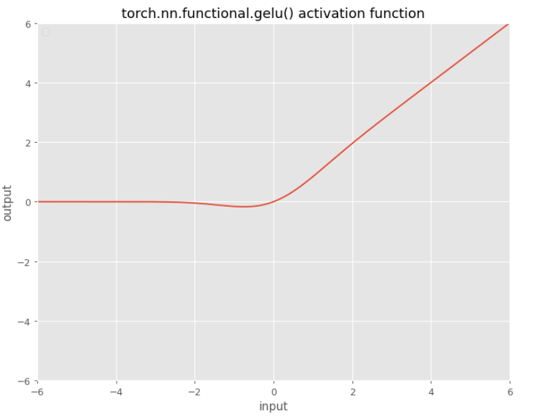
The Gaussian Error Linear Unit, or GELU is $x\Phi(x)$, where $\Phi(x)$ is the standard Gaussian cumulative distribution function.
One can approximate the GELU with: $0.5x\left(1+\tanh\left[\sqrt{2/\pi}\left(x + 0.044715x^{3}\right)\right]\right)$ or $x\sigma\left(1.702x\right),$ but PyTorch’s exact implementation is sufficiently fast such that these approximations may be unnecessary.
GELUs are used in GPT-3, BERT, and most other Transformers.
Sigmoid
$f(x)=\Large \frac{1}{1+e^{-x}}$
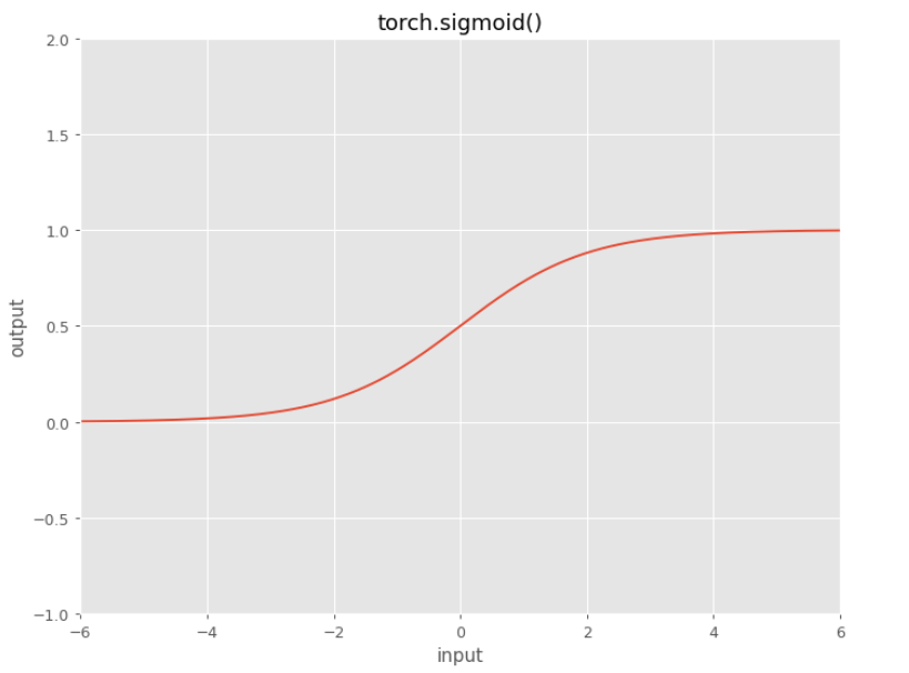
Drawback: sharp damp gradients during backpropagation from deeper hidden layers to inputs, gradient saturation, and slow convergence.
Derivative of this function is:
$f(x)’ = f(x)(1-f(x))$
Note we got the following output:
gradient at point 1: 0.1965664984852067
gradient at point 20: 2.0601298444944405e-09
Look how the second gradient at point x=20 is almost 0. Multiplying that number with the similar small number would produce what is called the computational instability. In this case vanishing gradient problem.
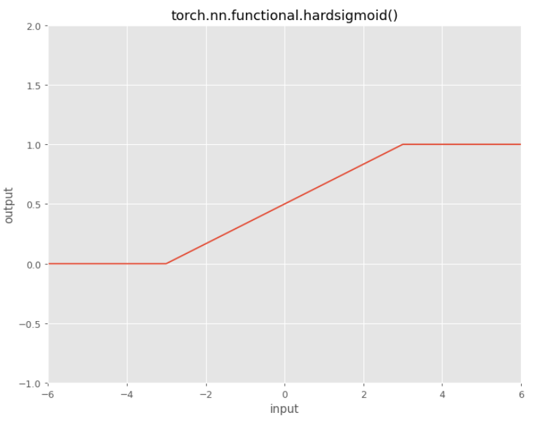
Hard Sigmoid
This function just tries to mimic the sigmoid.
Tanh
$f\left(x\right) = \large \frac{e^{x} - e^{-x}}{e^{x} + e^{-x}}$
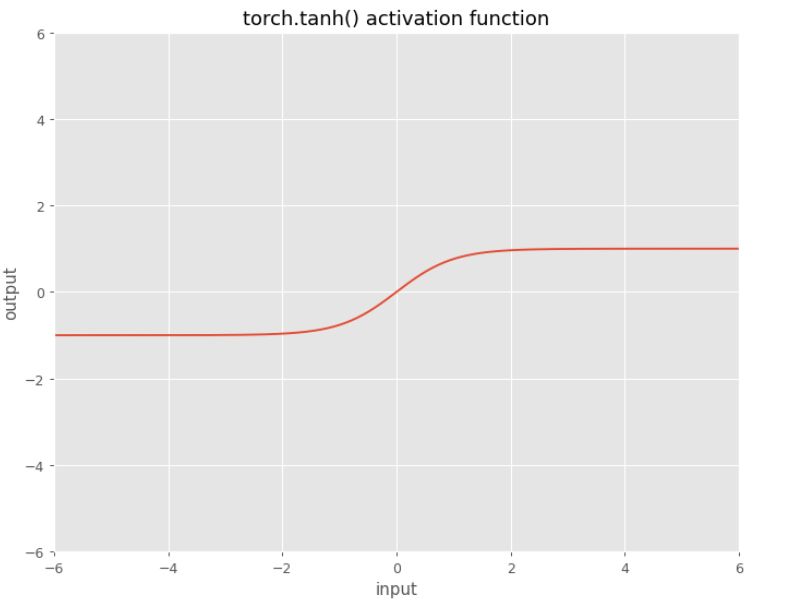
The tanh() activation function became preferred over the sigmoid function as it gave better performance for multi-layer neural networks. You can expect the output from this function to be close to zero mean.
Derivate: $f(x)’ = 1-f(x)^2$
Example: The difference between sigmoid and tanh
If you stack multiple layers with sigmoid nonlinearity the means of your outputs will be greater in the successive layers.
As a consequence you may not learn efficiently, and the system may not converge. This is why you need to pay attention to normalization.
With tanh() this is not the case, because the output mean should be around zero.
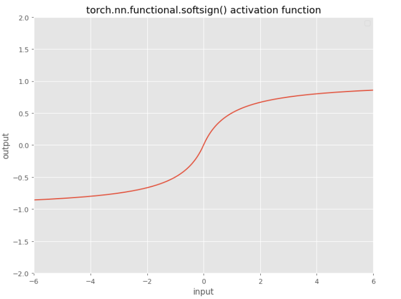
SoftSign
$f(x)=\frac{x}{1+ \mid x \mid}$
This function is proposed by Bengio. It is like a tanh() but it doesn’t go to the asymptotes as fast as tanh().
HardTanh
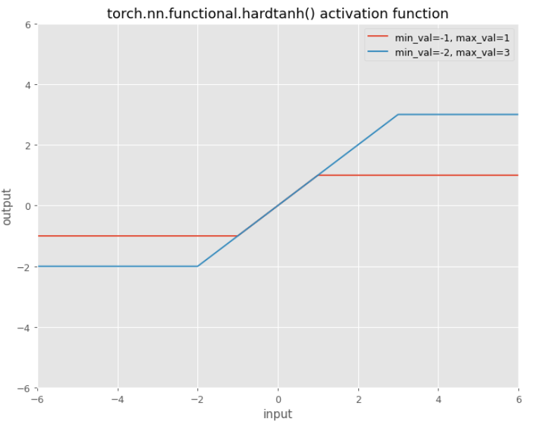
Default values:
min_val=-1max_val=1
You can tweak and use some other values.
Swish
$f(x) = \Large \frac{x}{1+e^{-\beta x}}$
Here $\beta$ is a learnable parameter. Nearly all implementations do not use the learnable parameter $\beta$, in which case the activation function is $x\sigma(x)$ (“Swish-1”).
The function $x\sigma(x)$ is exactly the SiLU introduced from GELUs paper.
Softplus
$f(x) = \ln \left(1+e^{x}\right)$
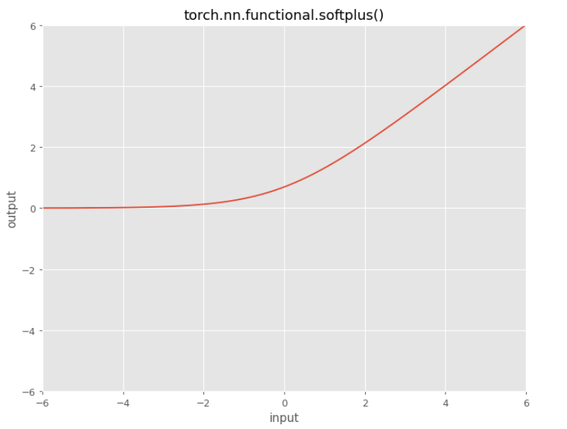
It can be viewed as a smooth version of ReLU, or differentiable version of ReLU.
The derivative which is exactly the sigmoid function:
$f(x)=\Large \frac{1}{1+e^{-x}}$
In PyTorch there are two more params you can tweak:
- beta=1
- threshold=20
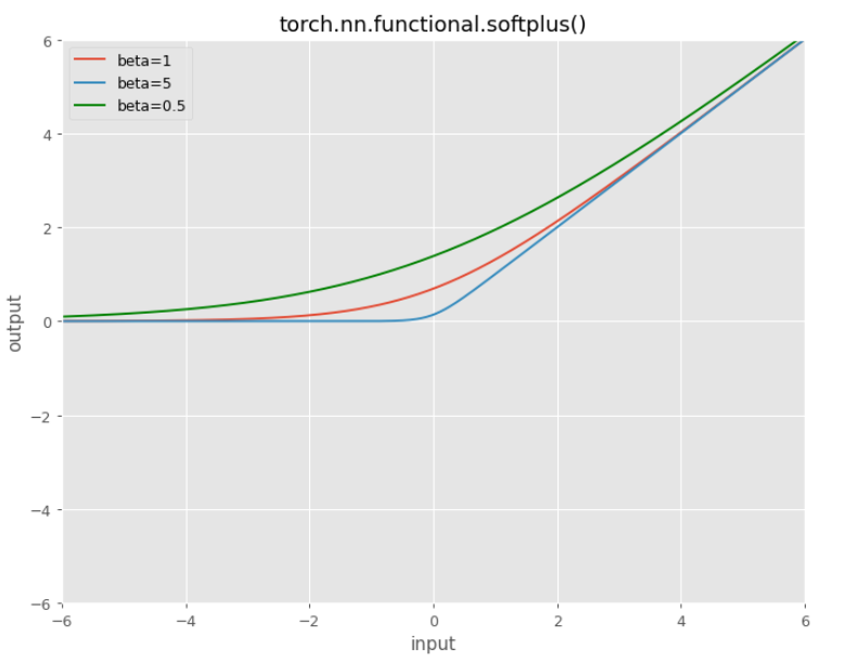
The scaling parameter $\beta$:
$f(x)=\frac{1}{\beta} * \ln (1+e^{\beta x})$
The larger $\beta$ the more the function will look like a ReLU.
To gain numerical stability the implementation reverts to the linear function when $\mathsf {input} \times \beta> \mathsf{threshold}$.
The higher the value of $\beta$ softplus() will be “much closer” to ReLU.
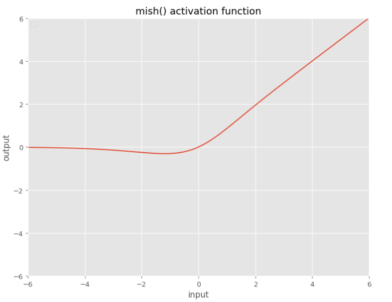
Mish
$f\left(x\right) = x\cdot\tanh{\text{softplus}\left(x\right)}$
where
$\text{softplus}\left(x\right) = \ln\left(1+e^{x}\right)$
You can define it in PyTorch:
def mish(x):
    return x*torch.tanh(torch.nn.functional.softplus(x))