CNNs
CNNs invented by Yann LeCun in 1989 became popular for image recognition tasks. Historically CNNs are great for both audio and image tasks, but could be applied also to a wide range of tasks involving complex data including: NLP, serial analysis, video analysis, etc.
Image tasks
When dealing with image classification of big images CNNs are a much better solution than plain fully connected neural networks (FCNN) because CNNs are memory efficient compared to FCNN.
The Imagenet challenge determined the historical evolution of CNNs starting from the AlexNet model.
The key feature traditional CNNs have is they are equivariant with respect to translation. This means if you have the cat on an image, the CNN will recognize the cat no matter where the cat is positioned if the cat is not rotated. This is an important feature that made CNNs practical for modern image tasks: image segmentation, object detection, image captioning, object classification, … no matter where the object is located in the image.
You can construct special CNNs that are equivariant wrt. rotation. These CNNs can recognize rotated objects.
Instead of term equivariant some sources also use the term invariant.
CNNs have filters. These filters are what CNNs learn. Two important things:
- multiple filters for each convolution layer
- convolutional filters share parameters
Mimicking the human brain
“Curse of dimensionality” is just a fancy name for the fact that images live in high dimensional vector spaces.
CNNs were able to find the solution for this curse by mimicking the human brain. This was evident after the Study of the Visual Cortex from Hubel and Wiesel (1964).
This work was so impactful that they won the Nobel prize in 1981.
Features Volume and Features Map
For the input image of volume 224x224x3 we would like to apply 64 filters of size 5x5. What will we get at the end of the convolution layer?
The volume we get is called activation volume or feature volume.
Single layer of this volume is called activation map or feature map.
To calculate the size of the activation map we need to convolve with each filter of size 5x5 over all possible inputs of size 5x5 to get the features.
You will get the new activation map of size: 224-5+1=220px. The result will be a bit different if we involve the padding.
The padding means we put the pixels with 0 value to the image border. If we use 2px padding the original 224px image will become 228px image because the 2px addition will be added both sides.
Now the calculus changes a little bit. The new receptive field will become:
224+2*2-5+1=224px
There is stride we may involve. Stride means we move our filter S pixels each time. In case stride=2 the calculus has the final form:
$W_o = (W_1+2*P-F_w)/S+1$
$H_o = (H_1+2*P-F_h)/S+1$
The formula may become even more general if we involve the dilated convolution D in which case we have:*
$F = F + (F − 1)(D − 1)$.
Receptive field
Receptive field is the imaginary region of the input image that affects the activation of a feature. It is per feature, so it is the region that the feature is looking.
Example: Calculate the receptive field of VGG16
We will use the following formulas:
$n_{out} = \lfloor\frac{n_{in}+2p-k}{s}\rfloor+1$
$j_{out} = j_{in}*s$
$RF_{out} = RF_{in}+(k-1)*j_{in}$
Where $n$ denotes the number of out features per spatial dimension. In case we deal with CIFAR-10 it will be 32 at the start.
$j$ is a jump it is how stride affects the receptive field $RF$.
Notice that the $RF$ doesn’t depend on $n$, but it depends on stride $s$ and kernel size $k$ that we can find just in convolution and max pooling layers.
| # | name | n | j | RF |
|---|---|---|---|---|
| 0 | input | 32 | 1 | 1 |
| 1 | conv1_1 | 32 | 1 | 3 |
| 2 | conv1_2 | 32 | 1 | 5 |
| 3 | maxpool | 16 | 2 | 6 |
| 4 | conv2_1 | 16 | 2 | 10 |
| 5 | conv2_2 | 16 | 2 | 14 |
| 6 | maxpool | 8 | 4 | 16 |
| 7 | conv3_1 | 8 | 4 | 24 |
| 8 | conv3_2 | 8 | 4 | 32 |
| 9 | conv3_3 | 8 | 4 | 40 |
| 10 | maxpool | 4 | 8 | 44 |
| 11 | conv4_1 | 4 | 8 | 60 |
| 12 | conv4_2 | 4 | 8 | 76 |
| 13 | conv4_3 | 4 | 8 | 92 |
| 14 | maxpool | 2 | 16 | 100 |
| 15 | conv5_1 | 2 | 16 | 132 |
| 16 | conv5_2 | 2 | 16 | 164 |
| 17 | conv5_3 | 2 | 16 | 196 |
| 18 | maxpool | 1 | 32 | 212 |
| 19 | adaptivepool | 1 | 32 | 212 |
| 20 | linear | 1 | 32 | 212 |
The number of parameters of Convolution layer
To calculate the number of parameters for the conv layer on the input 224x224x3 where the filter is 5x5 and there are 64 filters we use the formula:
3*5*5*64+64
We add 64 because there are 64 filter biases and the rest just multiplication of the input and output volumes and the filter size.
Meaning of parameters
Explain nn.Conv2d(3,10, 2,2) numbers 3 and 10 in PyTorch?
The in_channels in the beginning is 3 for images with 3 channels (colored images). For images black and white it should be 1. Some satellite images may have 4 in there.
The out_channels is the number of convolution filters we have: 10. The filters will be of size 2x2.
Should we use bias in conv2d?
It is possible to use bias, but often it is ignored, by setting it with bias=False. This is because we usually use the BN behind the conv layer which has bias itself.
Empirically in a large model, removing the bias inputs makes very little difference because each node can make a bias node out of the average activation of all of its inputs, which by the law of large numbers will be roughly normal.
Setting bias=False in PyTorch
nn.Conv2d(1, 20, 5, bias=False)
Why do we use pooling layers in CNNs?
One of the reasons to use pooling layers is to increase the receptive field and to reduce the size of feature maps.
With each convolution layer increase the number of filters and lower the features maps to keep the same number of features throughout the architecture.
What is dilation?
To explain dilation take these two images:
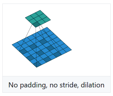
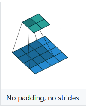
Without dilation all the neighboring pixels are taken to create new pixel in the activation map. With dilation half of the pixels are taken from the input image.
Transposed Convolution or Deconvolution terms
Deconvolution is mathematically defined as the inverse of a convolution.
In computer vision transposed convolution or strided convolutions sometimes is also called deconvolution.
We know the inverse operation is not the same as transpose operation so it is better to call it transposed convolution.
Why a 3x3 filter is the best.
According to the paper from Max Zeiler.
Tips on convolution
- Convolution is position invariant and handles location, but not actions.
- In PyTorch convolution is actually implemented as correlation.
- In PyTorch
nn.ConvNdandF.convNddo have reverse order of parameters.
Bag of tricks for CONV networks
This Bag of tricks paper presents many tricks to be used for Convolutional Neural Networks such as:
- Large batch training
- Low precision training
- Decay of the learning rate
- Resnet tweaks
- Label smoothing
- Mixup training
- Transfer learning