Softmax vs. Sigmoid functions

In Machine Learning, you deal with softmax and sigmoid functions often. I wanted to provide some intuition when you should use one over the other.

Suppose you have predictions as the output from a neural net.

These are the predictions for cat, dog, cow, and zebra. They can be positive or negative (no ReLU at the end).

Softmax

If we plan to find exactly one value we should use the softmax function. The character of this function is “there can be only one”.

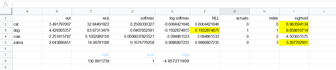
Note the out values are in the B column. Then for each B value $x$ we create $e^x$ in column C.

What the exp function do it will do:

it will make the predictions positive
what ever was max, it will stand out as max

The softmax function:

\[softmax( x_i ) = { e^{x_i} \over \sum_{j=1}^k { e^{x_j} } }\]

Can be literally expressed as taking the exponent value and dividing it by the sum of all other exponents. This will make one important feature of softmax, that the sum of all softmax values will add to 1.

Just by peaking the max value after the softmax we get our prediction.

Sigmoid

Things are different for the sigmoid function. This function can provide us with the top $n$ results based on the threshold.

If the threshold is e.g. 3 from the image you can find two results greater than that number. We use the following formula to evaluate the sigmoid function.

\[sigmoid( x ) = { e^{x} \over 1+ e^{x} }\]

Exactly, the feature of sigmoid is to emphasize multiple values, based on the threshold, and we use it for the multi-label classification problems.

And in PyTorch…

In PyTorch you would use torch.nn.Softmax(dim=None) to compute softmax of the n-dimensional input tensor. Here I am rescaling the input manually so that the elements of the n-dimensional output tensor are in the range [0,1].

import torch.nn as nn
m = nn.Softmax(dim=0)
inp = torch.randn(2, 3)*2-1
print(inp)
 
out = m(inp)
print(out)
print(torch.sum(out))
 
# tensor([[-1.2928, -2.9990, -1.8886],
#         [ 0.1079, -3.6320, -1.6835]])
# tensor([[0.1977, 0.6532, 0.4489],
#         [0.8023, 0.3468, 0.5511]])
# tensor(3.)
 

Note you need to specify the dimension for softmax, which is dim=0 in the previous example (dimension of columns). This is why the total sum will add to 3. since we have three columns.

But we can also use the functional version of softmax. The previous example can be rewritten as:

import torch.nn.functional as F
inp = torch.randn(2, 3)*2-1
print(inp)
out = F.softmax(inp, dim=0)
print(out)
print(torch.sum(out))
 
# tensor([[ 0.9096, -2.5876, -2.2403],
#         [-0.8566,  0.2757, -1.9268]])
# tensor([[0.8540, 0.0540, 0.4223],
#         [0.1460, 0.9460, 0.5777]])
# tensor(3.)

There is also a special 2d softmax that works on 4D tensors only, but you can always rewrite it using the regular F.softmax.

m = nn.Softmax2d()
inp = torch.randn(1, 3, 2, 2)
out = m(inp)
out2 = F.softmax(inp, dim=1)
 
print(torch.equal(out, out2)) #True

For the sigmoid function the things are quite clear, based on logits we get probabilities.

inp = torch.randn(1,5)
print(inp)
print(F.sigmoid(inp))
# tensor([[-0.4010,  0.0468, -0.4071,  0.6252,  1.0899]])
# tensor([[0.4011, 0.5117, 0.3996, 0.6514, 0.7484]])

Single vs. multi-label classification

We should use softmax if we do classification with one result, or single label classification (SLC). We should use sigmoid if we have a multi-label classification case (MLC).

Case of SLC:

Use log softmax followed by negative log likelihood loss (nll_loss). Here is the implementation of nll_loss:

def nll_loss(p, target):
    return -p[range(target.shape[0]), target].mean()

There is one function called cross entropy loss in PyTorch that replaces both softmax and nll_loss.

lp = F.log_softmax(x, dim=-1)
loss = F.nll_loss(lp, target)

Which is equivalent to :

loss = F.cross_entropy(x, target)

Do not calculate log of softmax directly instead use log-sum-exp trick:

def log_softmax(x): 
    return x - x.exp().sum(-1).log().unsqueeze(-1)

Case of MLC:

We use sigmoid and binary cross entropy functions in PyTorch that do broadcasting.

def sigmoid(x): return 1/(1 + (-x).exp())
def binary_cross_entropy(p, y): return -(p.log()*y + (1-y)*(1-p).log()).mean()

Sigmoid converts anything from (-inf, inf) into probability [0,1]. binary_cross_entropy will take the log of this probability later.

We can forget about sigmoids if we use F.binary_cross_entropy_with_logits function. This function takes logits directly.

F.sigmoid + F.binary_cross_entropy = F.binary_cross_entropy_with_logits

F.sigmoid will take logits and you may be careful in here in general case logit(sigmoid(x)) is not stable:

%matplotlib inline
import torch
torch.Tensor.ndim = property(lambda x: len(x.size()))
import matplotlib.pyplot as plt
x=torch.arange(-20, 20, 1e-4)
def sigmo(x):
    return 1/(1+torch.exp(-x))
 
def logit(x):
    return torch.log((x/(1-x)))
 
plt.plot(x, logit(x))
plt.xlabel("logit")
plt.show()
plt.close()
plt.plot(x, sigmo(x))
plt.xlabel("sigmoid")
plt.show()
plt.close()
plt.plot(x, logit(sigmo(x)))
plt.xlabel("logit(sigmoid(x))")
plt.show()
plt.close()
y = logit(sigmo(x))
plt.plot(x, ((y-x+1e-5)/(x+1e-3)))
plt.xlabel("(logit(sigmo(x)-x)/x")
plt.show()
plt.close()

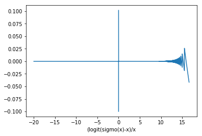
Still, the PyTorch implementation of F.binary_cross_entropy_with_logits should be numerically stable.

An example in SLC

batch_size, n_classes = 10, 5
x = torch.randn(batch_size, n_classes)
print("x:",x)
 
target = torch.randint(n_classes, size=(batch_size,), dtype=torch.long)
print("target:",target)
 
 
def log_softmax(x): 
    return x - x.exp().sum(-1).log().unsqueeze(-1)
 
def nll_loss(p, target):
    return -p[range(target.shape[0]), target].mean()
 
pred = log_softmax(x)
print ("pred:", pred)
ohe = torch.zeros(batch_size, n_classes)
ohe[range(ohe.shape[0]), target]=1
print("ohe:",ohe)
pe = pred[range(target.shape[0]), target]
print("pe:",pe)
mean = pred[range(target.shape[0]), target].mean()
print("mean:",mean)
negmean = -mean
print("negmean:", negmean)
loss = nll_loss(pred, target)
print("loss:",loss)