Impact of Weight Decay

Logistic Regression is a single linear layer (nn.Linear in PyTorch) neural network used with CrossEntropyLoss PyTorch criterion. We can write a custom module in PyTorch to create one.

class M(nn.Module):
    'custom module'
    def __init__(self):
        super().__init__()
        self.lin = nn.Linear(784, 10)
      
    def forward(self, xb):
        return self.lin(xb)

_{That would be Dense layer in TensorFlow.}

This neural network doesn’t even have a single activation function (F.relu or similar).

The main reason to analyse Logistic Regression is because it is simple.

The simplicity of this model can help us to examine batch loss and impact of Weight Decay on batch loss.

Here is the example using the MNIST dataset in PyTorch.

The model implements custom weight decay, but also uses SGD weight decay and Adam weight decay.

The example has a probe function allowing us to test different hyperparameters on the same model.

def probe(model, criterion, optimizer, bs, epochs, lr, wd_factor, color):

As you noted we provide:

• the model (our LR model)
• the criterion function which is always nn.CrossEntropyLoss() for our MNIST example,
• the optimizer, in fact I tested with both SGD, and Adam, but any optimizer can be used.
• the bach size, in here this is set to 64,
• the number of epochs, in here I examined a single epoch only,
• the learning rate (it depends if we will use the momentum or no),
• our custom weight decay factor wd_factor or 0 if we don’t plan to use custom WD
• and the color

The impact of the learning rate

First I examined the learning rate to find the one I should use with SGD:

criterion = nn.CrossEntropyLoss()
 
bs=64
epochs = 1
wd_factor = 0.0
 
lr = 0.1
model = M()
optimizer = torch.optim.SGD(model.parameters(), lr=lr)
probe(model, criterion, optimizer, bs, epochs, lr, wd_factor, "r") #red
 
lr = 0.01
model = M()
optimizer = torch.optim.SGD(model.parameters(), lr=lr)
probe(model, criterion, optimizer, bs, epochs, lr, wd_factor, "g") #green
 
lr = 0.001
model = M()
optimizer = torch.optim.SGD(model.parameters(), lr=lr)
probe(model, criterion, optimizer, bs, epochs, lr, wd_factor, "b") #blue

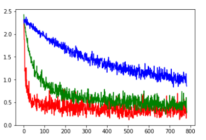
This image represents a single epoch. Note how the biggest learning rate (red) decreases the batch loss really fast, but oscillates stronger, compared to the blue.

At the end the cumulative epoch loss will be lower for the red so I decided to use lr=1e-1 (red learning rate)

Epoch 0 #red
Train loss: 0.3989532570761945
Validation loss: 0.2992929560662825
Epoch 0 #green
Train loss: 0.6678904935603251
Validation loss: 0.40658352872993375
Epoch 0 #blue
Train loss: 1.4549870281420705
Validation loss: 0.9654966373986835

Using Weight Decay 4e-3

From the Leslie Smith paper I found that wd=4e-3 is often used so I selected that.

The basic assumption was that the weight decay can lower the oscillations of the batch loss especially present in the previous image (red learning rate).

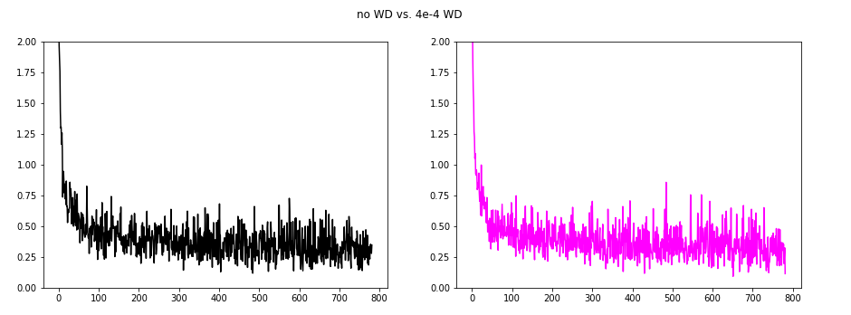
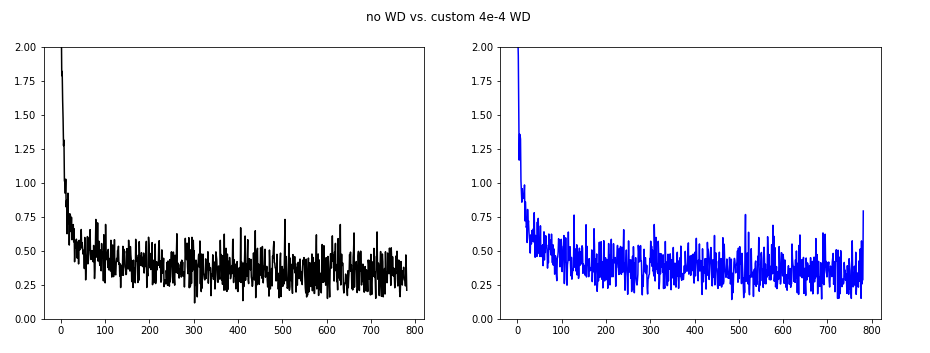
I first tried to understand the impact of weight_decay on SGD.

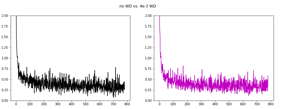
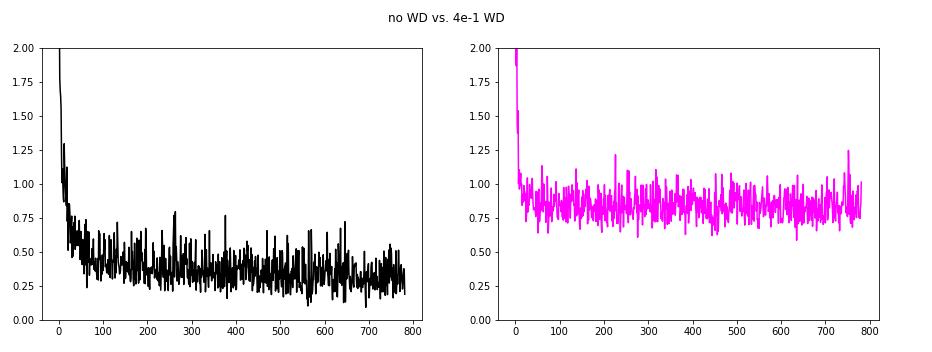
The left hand side shows the SGD with no WD (black), and the right side shows different SGD WDs:

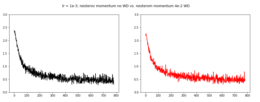
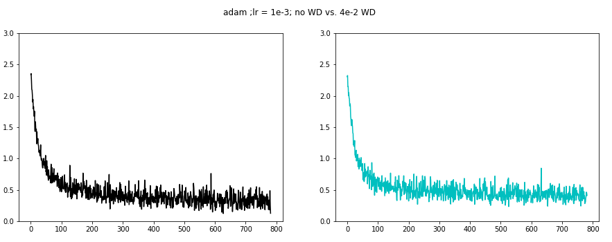
The next image compares no WD with 4e-2 WD.

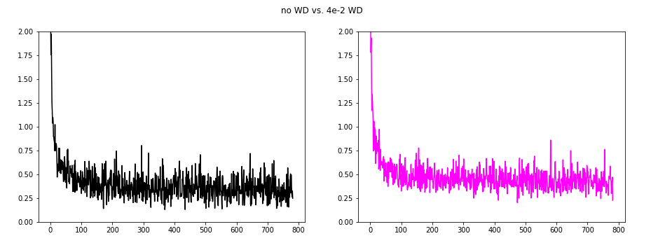
This really made some changes. The oscillations are reduced, but the loss increased a bit.

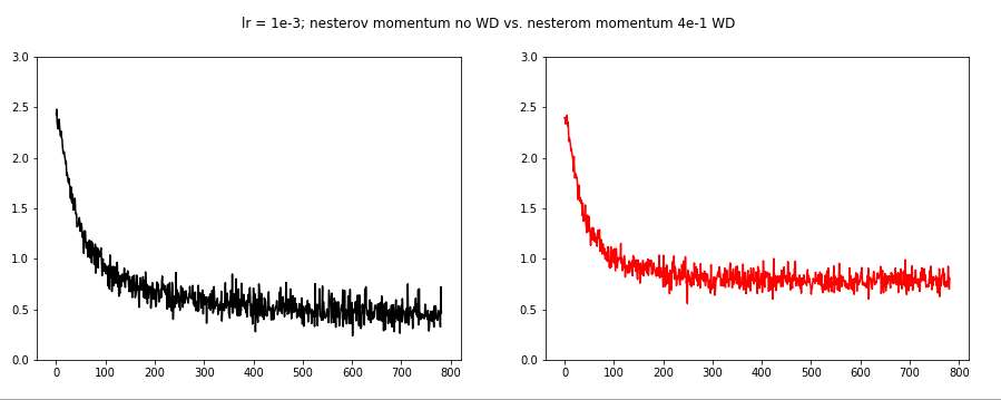
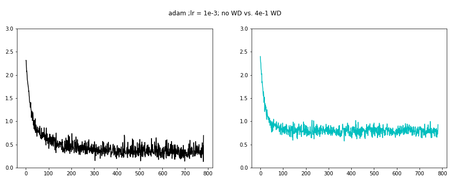
The very next image shows no WD vs. 4e-1 WD. We are kind of increasing the loss overall, and the oscillations are reduced.

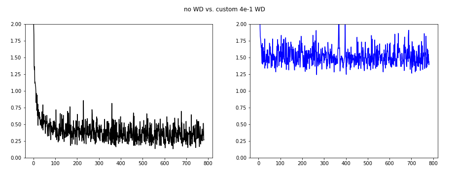
Now it is time to check the custom weight decay implemented like this:

wd = 0.
for p in model.parameters(): 
    wd += (p**2).sum()
loss = criterion(output, target)+wd*wd_factor 

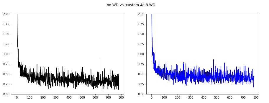
In blue are different WD values. We are on a single epoch with with SGD, and WD 1e-1:

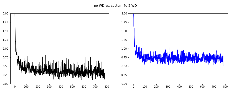
As we can see the oscillations are best suppressed for wd=4e-2.

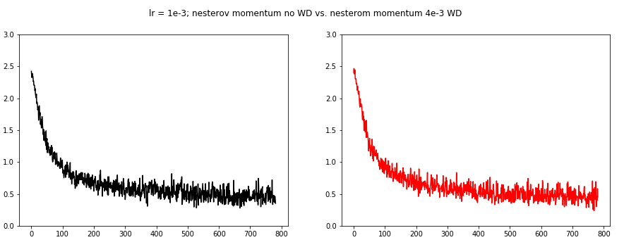
For the next three images we used the Nesterov momentum. However, we needed to decrease the learning rate to 1e-3 this time.

WD 4e-1 seams to decrease the batch loss oscillations.

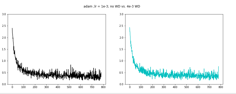
Finally we examine the Adam optimizer. Again we needed to lower the learning rate to 1e-3.

WD 4e-1 seams to decrease the batch loss oscillations.

Conclusion

For every optimizer there is a learning rate that works well for the first epoch.

At the same time there is a single WD value that really suppressed the oscillations.

Some low WD values do not have any impact, and some big WD values do hurt the loss decreasing.

This all leads to the idea there is an ideal WD value for the other specific optimizer setting including the lr.

Great for penalizing the big weights.

When the weight decay coefficient is big, the penalty for the big weights is also big, when it is small there is no such penalty.

Can hurt the performance at some point.

Weight Decay can hurt the performance of your neural network at some point.

Let the prediction loss of your net is $\mathcal{L}$ and the weight decay loss $\mathcal{R}$.

Given a coefficient $\lambda$ that establishes a tradeoff between the two.

At the optimum of this loss, the gradients of both terms will have to sum up to zero:

This makes clear that we will not be at an optimum of the training loss.

The higher $\lambda$ the steeper the gradient of $\mathcal{L}$, which in the case of convex loss functions implies a higher distance from the optimum.

Is why in this paper there are some studies that WD may even not be needed, especially when there are some other techniques to regularize the model.

_{Note: Weight Decay and L2 regularization are almost identical when the implementation is in question, the difference may be just a single factor of 2.}

Resources: 1 2, 3