Color Normalization
As you may assume in machine learning we can apply different normalization techniques.
Most obvious is to normalize the image that is represented as a sequence of bytes (values from 0 to 255) by dividing with 255. This is how all activation values will be inside interval [0,1].
However, better would be to touch both the mean and standard deviation. The following code will do this:
def normalize(x, m, s): return (x-m)/(s+1e-6)
def normalize_to(train, valid):
    m,s = train.mean(),train.std()
    return normalize(train, m, s), normalize(valid, m, s)
This would be for single channel images like in MNIST.
Here we calculated the train set mean and train set standard deviation (for all images inside the set).
But, there’s also multiple channels. That would be to normalize the images you have in your train, validation and test set for each channel.
These are for instance mean and std values for well known (RGB) image sets :
cifar_stats = ([0.491, 0.482, 0.447], [0.247, 0.243, 0.261])
imagenet_stats = ([0.485, 0.456, 0.406], [0.229, 0.224, 0.225])
...
Note: [0.491, 0.482, 0.447] is the mean for the cifar image set; 0.491 is the mean for the Red channel, and so on. The standard deviation for the same image set is represented with this list [0.247, 0.243, 0.261] and 0.247 is exactly the std of the Red channel.
The procedure in practice:
With PyTorch you will often use the PIL Image class to convert the image to PyTorch tensor.
from PIL import Image
from torchvision.transforms import ToTensor
Our Tensor images will look like this after the conversion:
tensor([[[0.1725, 0.2353, 0.2941,  ..., 1.0000, 1.0000, 0.9843],
         [0.1804, 0.2314, 0.2824,  ..., 1.0000, 1.0000, 0.9843],
         [0.1922, 0.2314, 0.2706,  ..., 1.0000, 1.0000, 0.9843],
         ...,
         [0.7098, 0.6863, 0.6627,  ..., 0.6863, 0.6863, 0.6039],
         [0.6941, 0.6824, 0.6745,  ..., 0.6118, 0.6314, 0.5569],
         [0.6863, 0.6863, 0.6941,  ..., 0.2392, 0.2902, 0.3137]], ...
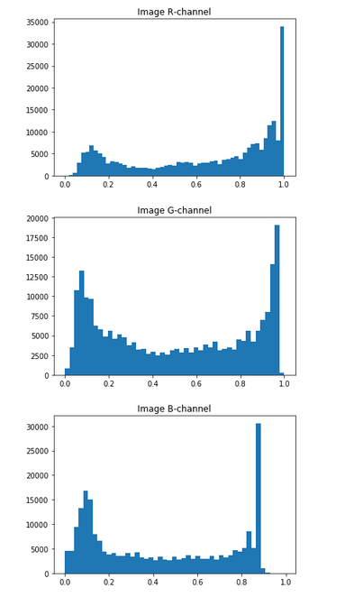
Note: min and max value of this tensor will be: tensor(0.) and tensor(1.) respectively.
Note: PIL library is not the fastest choice out there.
The histogram per channel will look like this:
…
Let we use the following PyTorch color normalization function:
def normalize(x: torch.FloatTensor, mean: torch.FloatTensor, std: torch.FloatTensor) -> torch.FloatTensor
    "Normalize `x` with `mean` and `std`."
    return (x - mean[..., None, None]) / std[..., None, None]
Note the Ellipsis notation we used inside the normalize function. It may be strange what it means in PyTorch.
Let’s check this code:
l=Tensor([1,2,3])
print(l)
r=l[...,None, None]
print(r)
This will output like this:
tensor([1., 2., 3.])
tensor([[[1.]],
        [[2.]],
        [[3.]]])
Note how we subtract x - mean[..., None, None] for a specific RGB channel, and also how we do RGB channel division std[..., None, None] after that.
At the end, we will get the result like this where our data pixel values will be around 0.
…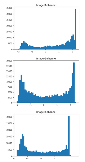
You may note that before we had our pixel values inside [0., 1.] range, and now we have positive and negative values around 0, ideal for machine learning.
This last case is used when you need to normalize the whole dataset, not just the single image.
On GPU
Also here is how to do normalization on the GPU for the Imagenet.
mean = torch.Tensor([0.485, 0.456, 0.406]).float().reshape(1,3,1,1)
std = torch.Tensor([0.229, 0.224, 0.225]).float().reshape(1,3,1,1)
print(mean)
print(std)
On GPU based on batch data
t = torch.rand(2,3,2,2)
t.cuda()
print(t)
# mean = t
m = t.mean((0,2,3), keepdim=True)
s = t.std((0,2,3), keepdim=True)

print(m, m.size())
print(s, s.size())
# let's normalize

t = (t-m)/(s+1e-6)

print(t)

m = t.mean((0,2,3), keepdim=True)
s = t.std((0,2,3), keepdim=True)

print(m, m.size())
print(s, s.size())