Batch normalization is the regularization technique for neural networks presented for the first time in 2015 in this paper.

The paper explains the regularization effect, explains the improvements and tries to provide the clue why it works.

Achievement

Thanks to the batch norm for the first time the ImageNet exceeded the accuracy of human raters, and stepped the era where machine learning started to classify images better than humans (for the particular classification task).

This is why we may call Batch Normalization (BN) a milestone technique in the development of deep learning.

How it works in PyTorch?

There are few things important for the batch norm (BN):

BN is to be applied to every mini-batch (mb).
For each feature $c_i$ (from C features) in the mini-batch (mb), BN computes the mean and variance of that feature. This means batch normalization normalizes the input for each channel independently.
BN will then normalize each feature $c_i$, by subtracting the mean μ and will divide by standard deviation σ of that feature.
If we have affine=False we will have what we stated so far.
If we have affine=True we will have two more learnable parameters β and γ. γ is the slope (weight) and β is the intercept (bias) for the affine transformation. These parameters are learnable and initially they will be set to all zeros for β and all ones for γ.

Example:

import torch
import torch.nn as nn
m_a = nn.BatchNorm1d(10, affine=True)

input = 1000*torch.randn(3, 10)
print(input)
output = m_a(input)
print(output)
for name, param in m_a.named_parameters():
    print(name, param)

for name, param in m_a.named_buffers():
    print(name, param)

In here input had 3 channels and 10 features.

Output:

tensor([[ 1189.5525,   783.1801,  1783.5414,  -104.5690,  -891.8502,   237.1147,
           711.3362,   836.8916,  -200.6111,   692.7631],
        [-1208.0027, -1255.1088,    29.4310, -1918.3954, -1294.7596,   955.5003,
          -752.8644,  -825.5052,  -771.2104,   321.2602],
        [  977.7232,  -480.7817,  1928.1239,   675.1355,  -332.6682,  -274.7805,
         -1350.9822, -1380.2109,  -264.8417,  -161.7669]])
tensor([[ 0.8026,  1.3103,  0.6217,  0.3173, -0.1320, -0.1364,  1.3569,  1.3727,
          0.8292,  1.1682],
        [-1.4097, -1.1160, -1.4109, -1.3522, -1.1534,  1.2872, -0.3332, -0.3920,
         -1.4067,  0.1063],
        [ 0.6071, -0.1943,  0.7892,  1.0349,  1.2854, -1.1508, -1.0236, -0.9808,
          0.5775, -1.2744]], grad_fn=<NativeBatchNormBackward>)
weight Parameter containing:
tensor([1., 1., 1., 1., 1., 1., 1., 1., 1., 1.], requires_grad=True)
bias Parameter containing:
tensor([0., 0., 0., 0., 0., 0., 0., 0., 0., 0.], requires_grad=True)
running_mean tensor([ 31.9758, -31.7570, 124.7032, -44.9276, -83.9759,  30.5945, -46.4170,
        -45.6275, -41.2221,  28.4085])
running_var tensor([176176.5781, 105864.2891, 111714.9297, 177072.7031,  23344.9102,
         38195.9883, 112580.6562, 133114.3281,   9769.5420,  18360.0840])
num_batches_tracked tensor(1)

With affine=True we multiply normalized output by parameter called weight and add to that the parameter bias.
If we set track_running_stats=True in PyTorch running statistics will be calculated and BN output will be less bumpy; this is by default.
If we set track_running_stats=False the previous output will not have the running_mean tensor and running_var tensor.

Simplified (without using the running statistics) we can express this as:

\[y = n(f(w_1, w_2, ... w_n, x)) * weight + bias\]

Where $n$ is the normalization function, $weight$, and $bias$ are our scale and offset parameters, $f$ is our function to create the output from the layer, $x$ and $y$ are the activations.

\[y = f(w_1, w_2, ... w_n, x)\]

After the normalization we have the the mean of 0 and standard deviation of 1 for the single batch. Here is the example:

import torch
import torch.nn as nn

# affine=False means nothing to learn
m = nn.BatchNorm1d(10, affine=False,track_running_stats=False)
input = 1000*torch.randn(3, 10)
print(input)
output = m(input)
print(output)
print(output.mean()) # should be 0
print(output.std()) # should be 1

PyTorch class _BatchNorm explains clearly we use the parameters weight and bias if we set self.affine=True :

if self.affine:
    self.weight = Parameter(torch.Tensor(num_features))
    self.bias = Parameter(torch.Tensor(num_features))
else:
    self.register_parameter('weight', None)
    self.register_parameter('bias', None)
if self.track_running_stats:
    self.register_buffer('running_mean', torch.zeros(num_features))
    self.register_buffer('running_var', torch.ones(num_features))
    self.register_buffer('num_batches_tracked', torch.tensor(0, dtype=torch.long))
else:
    self.register_parameter('running_mean', None)
    self.register_parameter('running_var', None)

Parameters and Buffers in PyTorch

Couple things to cover from the previous code:

There is a concept of module parameter (nn.Parameter). Parameter is just a tensor limited to the module where it is defined. Usually it will be defined in the module constructor (__init__ method).

register_parameter method in previous code will do some safe checks before set the parameter to None, meaning we will not learn the values of weight and bias if self.affine is not True.

Once we have module parameter defined, it will appear in the module.parameters().

There is also a concept of buffer in PyTorch.

register_buffer is specific tensor that can go to GPU and that can be saved with the model, but it is not meant to be learned (updated) via gradient descent. Instead it is calculated at every mini batch step.

As you may noted in PyTorch we have the training time and the inference time. While we train (learn/fit) we will constantly update the running_mean and running_var with the every mini batch. In the inference time we will just use the values calculated and we will not alter the running mean and var.

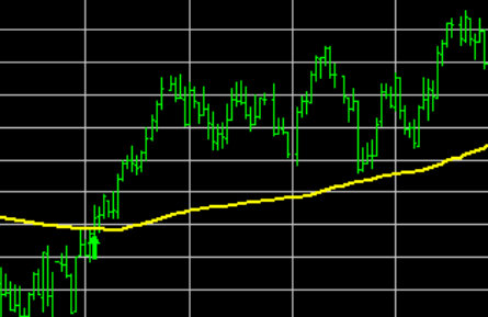
Note: running mean and running variance, are statistical methods calculating the moving average. What they essentially do you can spot from the image.

It is possible to use BN even if we set affine=False and track_running_stats=False. It will just work.

For completeness, batch norm is one of several norms. The other norms that exist:

Layer norm
Instance norm
Group norm

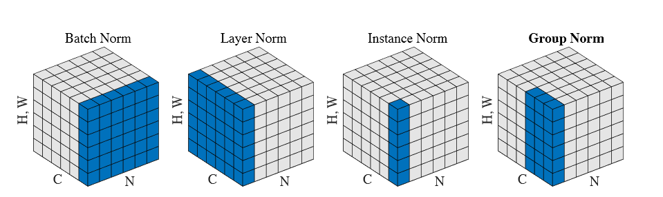
In the image each subplot shows a feature map tensor for an image related problem where:

$N$ as the batch axis
$C$ as the channel axis,
and $(H, W)$ as the spatial axes.

The pixels in blue are normalized by the same mean and variance, computed by aggregating the values of these pixels.

The presented image is little odd, because the spatial axes $H,W$ take just the single upward axis of the cube.

REFERENCE MATERIAL:

https://arxiv.org/abs/1502.03167
https://arxiv.org/pdf/1803.08494.pdf