PyTorch from tabula rasa
PyTorch is based on Torch. Torch is a Tensor library like Numpy. Unlike Numpy, Torch has strong GPU support.
You can use Torch either using the Lua programming language or if you like Python you can use PyTorch.
You can use PyTorch together with all major Python packages like scipy, numpy, matplotlib and Cython and benefit from PyTorch’s autograd system.
We will check some major PyTorch features in here and provide some feedback on PyTorch tensors, algebra and graphs.
Main PyTorch features
- Eager execution
- C++ support
- Native ONNX Support (Open Neural Network Exchange)
- Supported on major cloud platforms
- Supports all major network model architectures
Data types
We see in here the list of data types currently supported.
| Data type | Tensor |
|---|---|
| 32-bit floating point | torch.FloatTensor |
| 64-bit floating point | torch.DoubleTensor |
| 16-bit floating point | torch.HalfTensor |
| 8-bit integer (unsigned) | torch.ByteTensor |
| 8-bit integer (signed) | torch.CharTensor |
| 16-bit integer (signed) | torch.ShortTensor |
| 32-bit integer (signed) | torch.IntTensor |
| 64-bit integer (signed) | torch.LongTensor |
What do you do first in PyTorch?
In order to use it you first import the torch library.
import torch
Probable the next thing would be to convert your numpy arryas to PyTorch tensors
pta = torch.from_numpy(a)
The above line would also convert the original data type (DType) from numpy array. For example, float64 will become torch.DoubleTensor
We can also convert PyTorch tensor to numpy array:
a = pta.numpy()
We can override default behaviour if we cast it:
pta = torch.FloatTensor(a)
PyTorch tensor
Has three atributes:
torch.dtypetorch.devicetorch.layout
We already listed all dtype attrubutes in a section before. For the device we can have either “cpu” or “cuda”. Cuda is a software layer over hardware GPU unit. Currently it works only on Nvidia hardware. This “cuda” thing is what makes speed improvements.
A torch.layout is an object that represents the memory layout of a torch.Tensor. torch.strided means dense tensors. Experimental support for torch.sparse_coo exists.
You typically use the following ways to create the tensor in PyTorch:
- torch.Tensor(data)
- torch.tensor(data)
- torch.as_tensor(data)
- torch.from_numpy(data)
The privilege working with GPU
We can use both CPU and GPU with PyTorch. This would be how to move our data from CPU to GPU:
data = data.cuda()
Reshape the tensor
a = torch.range(1, 12)
a = a.view(3, 4)        # reshapes in 3 columns x 4 rows
Note you can use PyTorch reshape() method as well that will create the tensor copy if needed.
As we know, if we spec. the dimension -1 means dynamic dimension. In the next example this means all elements of tensor a, and that will make torch.Size([12]).
a.view(-1)
Basic Algebra in PyTorch
Here we define tensors a and b and do basic algebra operations:
a = torch.rand(4,4)
print(a)
b = torch.rand(4)
print(b)

mm = a.mm(a)       # matrix multiplication
mv = a.mv(b)       # matrix-vector multiplication
t= a.t()           # matrix transpose

print(mm)
print(mv)
print(t)
The output will be like this:
tensor([[0.9216, 0.0812, 0.3326, 0.1223],
        [0.4754, 0.1876, 0.8705, 0.0348],
        [0.8547, 0.2323, 0.1879, 0.7196],
        [0.0683, 0.3799, 0.8813, 0.9155]])
tensor([0.3089, 0.8028, 0.2625, 0.4179])
tensor([[1.1806, 0.2138, 0.5475, 0.4668],
        [1.2737, 0.2893, 0.5156, 0.7229],
        [1.1079, 0.4301, 1.1560, 0.9066],
        [1.0594, 0.6294, 1.3258, 1.4938]])
tensor([0.4883, 0.5404, 0.8006, 0.9401])
tensor([[0.9216, 0.4754, 0.8547, 0.0683],
        [0.0812, 0.1876, 0.2323, 0.3799],
        [0.3326, 0.8705, 0.1879, 0.8813],
        [0.1223, 0.0348, 0.7196, 0.9155]])
Also, we have Hadamard product with * and the dot product
a = torch.Tensor([[1,2],[3,4]])
b = torch.Tensor([5,6])
c = torch.Tensor([7,8])

print(a*b) # element-wise matrix multiplication (Hadamard product)
print(a*a)
print(torch.dot(b,c)) # not like in numpy, works just on 1D Tensors
Result
tensor([[ 5., 12.],
        [15., 24.]])
tensor([[ 1.,  4.],
        [ 9., 16.]])
tensor(83.)
The seed
We can set the torch seed using this line:
torch.manual_seed(seed)
We can set np.random.seed(seed) for the numpy library. This will help us set the deterministic results. Also note that Python programs need to set the hash seed in order to work deterministic.
The graph, the Variable, and the Function
The invasion of PyTorch tensors is becoming evident, but less evident is the idea of PyTorch variable and function. The interesting thing, if you try to print the variable you will get the output like you printed the Tensors. Let’s check this example:
import torch
from torch.autograd import Variable

def pr(obj):
  print(obj)
  print("type:", type(obj))

a = torch.Tensor([[1,2],[3,4]])
pr(a.grad_fn)
a2= a+2
pr(a2.grad_fn)
b = Variable(torch.Tensor([[1,2],[3,4]]), requires_grad=True)
pr(b.grad_fn)
b2 = b+2
pr(b2.grad_fn)
The output:
None
type: <class 'NoneType'>
None
type: <class 'NoneType'>
None
type: <class 'NoneType'>
<AddBackward0 object at 0x7f857dc19f60>
type: <class 'AddBackward0'>
b2 is a variable that has the function under .grad_fn that has created the variable.
The variable b we created doesn’t have the function that has created it, since we created it.
The complete history of computation is saved this way in the interconnected acyclic graph.
As we said the autograd package provides automatic differentiation for all operations in the graph so let’s check that next.
Autograd
What is PyTorch autograd?
The autograd package provides automatic differentiation for all operations on Tensors. This is needed for the backpropagation algorithm to work.
The import torch.autograd package is the heart of PyTorch. It contains classes and functions implementing automatic differentiation on a computation graph. Computational graph is what you get out-of-the-box in PyTorch once you set your computations.
Important things about the graph:
- when computing the forwards pass, autograd builds up a graph
- graph holds functions and variables (tensors)
- graph encodes a complete history of computation
- after the backward pass the graph will be freed to save the memory
- graph is recreated from scratch at every iteration (on forward pass)
- graph is needed to compute the gradients
Consider this small program:
# Create tensors
x = torch.tensor(1., requires_grad=True)
w = torch.tensor(2., requires_grad=True)
b = torch.tensor(3., requires_grad=True)

# Build the graph
y = w * x + b    # y = 2 * x + 3

# Compute gradients
y.backward()

# Print out the gradients.
print(x.grad)    # x.grad = 2
print(w.grad)    # w.grad = 1
print(b.grad)    # b.grad = 1
For the previous program:
- once we wrote the equation PyTorch creates computational graph on fly…
- every Tensor with a flag:
requires_grad=Fasewill freeze backward computation - every Tensor with a flag:
requires_grad=Truewill require gradient computation - when the forwards pass is done, we evaluate this graph in the backwards pass to compute the gradients.
y.backward()will do the backward pass- we used
.gradattribute to show the tensor gradient
PyTorch computes backward gradients using a computational graph which keeps track of what operations have been done during your forward pass.
In each iteration we:
- execute the forward pass,
- compute the derivatives of output with respect to the parameters of the network
- update the parameters to fit the given examples
After doing the backward pass, the graph will be freed to save memory. In the next iteration, a fresh new graph is created and ready for back-propagation.
The following program:
import torch
from torch.autograd import Variable
a = Variable(torch.rand(1, 4), requires_grad=True)
b = a**2
c = b*2
d = c.mean()
e = c.sum()
d.backward(retain_graph=True) # fine
e.backward(retain_graph=True) # fine
d.backward() # also fine
e.backward() # error will occur!
- creates a variable (tensor)
- creates new tensors from operations
- calls backward on
dandein turns - we compute derivatives once we call .backward() on a Tensor
- when ever we call
backward(retain_graph=True)the graph will still be in memory - once we called
d.backward()on leaf (graph element) graph will be removed - last call to
e.backward()will show the error that the graph has been removed from memory
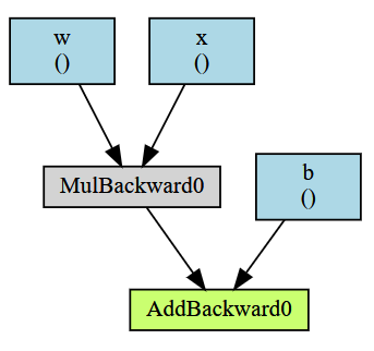
How to show the graphs?
I found a package torchviz (pip install torchviz) that prints the graphs. Our previous example will then become:
import torch
import torchviz
from torchviz import make_dot, make_dot_from_trace

print(torch.__version__)
# Create tensors.
x = torch.tensor(1., requires_grad=True)
w = torch.tensor(2., requires_grad=True)
b = torch.tensor(3., requires_grad=True)

# Build a computational graph.
y = w * x + b    # y = 2 * x + 3

# Compute gradients.
y.backward()

# Print out the gradients.
print(x.grad)    # x.grad = 2
print(w.grad)    # w.grad = 1
print(b.grad)    # b.grad = 1

make_dot(y, {'x': x, 'w':w, 'b': b})
Note how we set the names for the leaf graph elements inside the second make_dot parameter.
The output will be like this:
One another way to create the graphs is torch.jit.get_trace_graph.